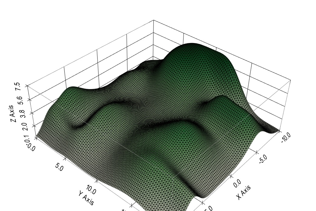
The needs of the neuroscientist overlap with the needs of the machine learning engineer in many ways. Visualization is important in both disciplines. For example, let's say we're looking at the effect of recurrent auto-excitation on Hopfield networks. We can look at the trajectories in the phase plane, and they show us a chaotic behavior. But what is that doing to the information? There are many reasons for controlling chaotic behavior, not the least of which is the "critical brain hypothesis". According to physical theory the boundaries of a critical region should exhibit power law behavior and fractal dynamics. Are we seeing those in the simulation? If so, how can we control them? And if not, why not? We'd like to visualize the energy surface of the Hopfield network under various conditions. A graph like this is "not bad", but it's old-school. How about a real-time animation, mapped to the cells of a mesh so it can be viewed in several different forms simultaneously?



How about linked graphs so as one rotates the network geometry, the power spectra rotate along with it? There are so many nice and powerful things one can do with the proper visualization! Ultimately the purpose of all this fancy simulation is information geometry, and in that area the visualization requirements are extreme. High dimensional data spaces are difficult to visualize, they require special tools. Some of them already exist in the data science community, some come from machine learning, and some come from organic demand on the part of biologists and psychologists. Meshes turn out to be simple low-dimensional expressions of higher dimensional graphs and simplicial structures. There are peculiarities in three dimensions, and there are also generalities that apply in any dimension. It's important to understand the geometry and the topology, both the locations of points and the ways they're connected. This is what allows us to use simple directives like DIVERGENCE 5 instead of having to provide the simulator with connection maps (which take a long time to build and tend to become error-prone, especially after midnight). There's no need for a connection map if you already you know you have topographic structures and you're just trying to find the nearest neighbors. The maps are generally used to represent oriented axons and dendrites, and even those don't require maps most of the time, as long as they can be represented with simple geometric transformations, and that requirement is well satisfied by ordinary biology in three dimensions. Before we jump in let's take a quick look at building synapses. So far we've seen CELLs, which are variously called "cell types" or "cell groups" or "sheets" or "layers" depending on the geometry, and we've seen NEURONs that are created from prototypes defined by the CELLs. But what about connections? Annie uses a CONNECTION object that works between cells. Connections are between CELLs, and synapses are between NEURONs. The CONNECTION object is a prototype synapse, it works just like a CELL except it parametrizes the synapse instead of the neuron. After a network build with 100 neurons, there could be tens of thousands of synapses, depending on how we specify the connectivity. Typically in rostral brain structures there will be "more than one" synapse between any two neurons, and we can tell Annie about this multiplicity and how to create it and control it.

To create a CONNECTION, you have to provide the "from" CELL and the "to" CELL, and you have to tell Annie what kind of connection it is - excitatory, inhibitory, gap junction, whatever - and you can add other qualifiers like BEHAVIOR, to give the synapse STDP capabilites and etc. Connections look like this in the network definition file:

CONNECTION NAME CONN FROM ON_BIPOLAR_CELLS TO A2_AMACRINE_CELLS
     DIVERGENCE (5,5,5)
     TYPE INHIBITORY
     BEHAVIOR STP
     WEIGHT 0.1
     TAU 0.05

And again, you can expand this definition at any level of detail you wish. You can tell Annie about the density of receptors, channels, and connexins in your synapse. You can tell her whether the synapse is built on spines, or whether it involves moduiators in addition to a primary neurotransmitter. Because the connection is named, you can then put the synapses into a capsule or wrap them with an astrocyte. It's this easy:

GLIA TYPE ASTROCYTE NAME A1
     WRAP CONN

You can also do:

CAPSULE GLOM NAME G
     INCLUDE CONN
     INCLUDE A1

You now have a glomerulus wrapped by the process of an astrocyte. Okay okay, there's a few more details, but that's basically the gist of it. When you do it this way, Annie will load in a pile of defaults. They'll work, although usually you'll want to provide some detail. One way to do it is, create the skeleton in a definition file and then use the interactive dashboard to fill in the details. Everything in Annie is a mesh, so when she shows you your synaptic capsule, you'll be able to position NMDA receptors anywhere you want. As you saw on the previous page, the meshes that Annie uses are way more resolute than anything you'll need for positioning purposes. (Take a look at the expanded axon again, you'd have to pick a vertex to attach a channel - could you do it? I'd have to zoom in at least another three times, otherwise I'd risk picking the wrong vertex). And to reiterate, if you want less resolution simply decrease the mesh density. You can reformat meshes inside Annie, or use Blender or 3DS or any of your favorite mesh tools. There's a bit of learning curve in handling meshes, but after a day or two you'll discover it's easy. And anytime you want, you can make the meshes disappear entirely and Annie will show you the ordinary shaded surfaces.

So, on to simulations. Visualization is the big deal in simulations. For example, here is a nice report from the 2018 time frame.


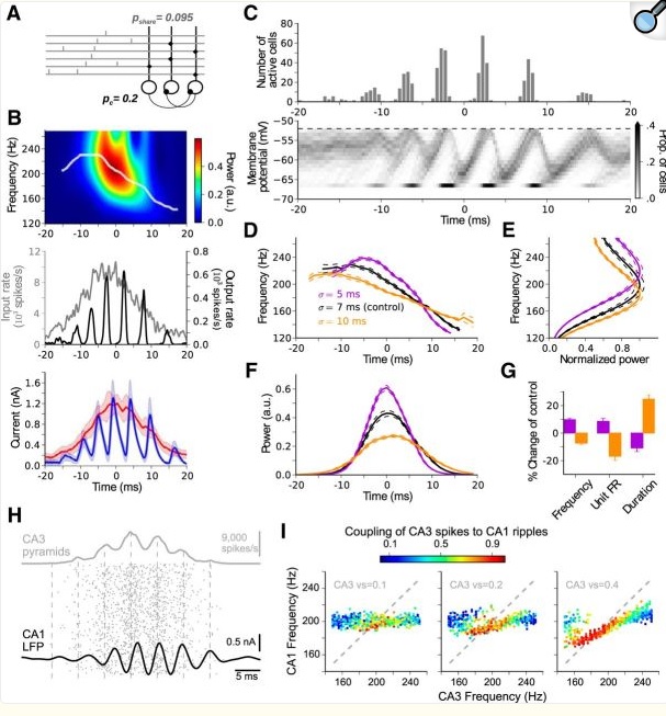
(from Donoso et al J Neurosci 38(12):3124)

Someone did a lot of work to get these graphs. This is a simulation investigating the role of inhibitory interneurons in hippocampal spindles, and in 2018 it was still difficult to shade a graph like their figure (C). It shouldn't be this hard, and we need to take it to the next level. Today, I can throw together any old network with a few excitatory and inhibitory neurons, and Annie will show me their I-f curves and let me manipulate them, she'll show me the population activity in the phase plane, and innumerable visualizations of type (B) that let me see hot-cold maps of network activity, that kind of thing. All this should be instantly available in real time, on-screen. It used to take months to put together a simulation like this, with Annie it can be done in 5 minutes. In this particular case it turns out the parameters don't matter much, you'll get pretty much the same behavior with a wide spectrum of weights and currents. But loose statements like this are not enough, everything has to be quantified. The statistics alone are a swamp, these days you practically have to be a data scientist to publish a paper. The good news is, everything is free and open-source and it just needs to be collected in one central place so you don't have to jump through hoops to test an hypothesis. The hierarchy of function from molecules to networks needs to be seamless. In the above simulation there was no recurrent connection from the inhibitory neurons back to the excitatory pyramidal cells. Why not? What happens when you add one? How can I control the dynamic between the spindle and fast gamma frequencies? Can I do it by adding a few synapses somewhere? Maybe changing an ion channel or two? What about these bursts? The latest research says they have information content, they talk to the polar orbitofrontal cortex in multiple-choice situations when an optimal response needs to be selected. A simulation has to do a lot more than just show me waveforms. We already know that just about anything is possible in neural networks, the purpose of simulations is not to say "look, it can be done". Most of the time, neuroscientists are interested in evaluating theory against biological reality. The engineering of it can get pretty specific, like in the above paper they're talking about a change in frequency resulting from population activity. These are the kinds of things we need to quantify and visualize, and the reality is, the math around it is every bit as complicated as fluid dynamics. The simplistic approach of integrate-and-fire neurons is old news by now (even though it's still very useful, but biological reality demands more).

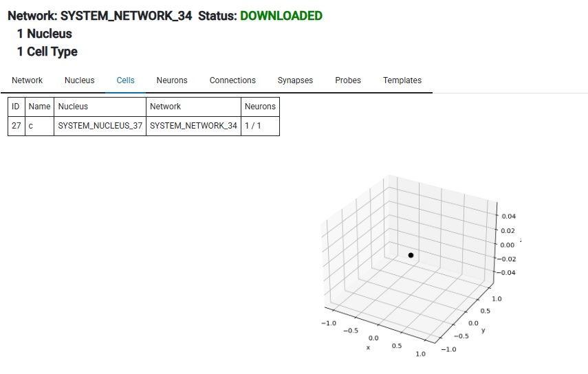
Let's start real simple, in the interactive dashboard. We'll create one neuron, with one synapse, and look at it. To do this, we'll be using the drop-down menu buttons on the right side of Annie's dashboard. The sequence of activity is: first:

Create Cell, name = 'C', type = External, N_Neurons = 1, Center=(0,0,0), Extent = (1000,1000,0), Arrangement=GRID_2D

This gives us exactly one neuron at location (0,0,0). Next we connect it to itself:

Create Connection, From C to C, Type = Inhibitory, Weight = 0.1, Tau = 0.05, Divergence = 1

Then push the Build Network button, then Download. Now you have a network in your workstation. It has one neuron in it. Here it is:



Next we do Create Simulation, followed by Add Network To Simulation. Now we need a stimulus of some kind, so we can either create one or load one from a file. I happen to have a file lying around, so I'll just load that.

Load Template File, name='CONES2.TEM' - which happens to have a convenient sin wave generator called T2 (it's the same one shown earlier!). So now,

Create Apply, Template = 'T2', Cell = C

And finally, to get some output, we create a Probe and put it on the CELL.

Create Probe, probe_type = Level, probe_object = C, file = 'test_probe.out'

And now we push the Start button, wait for a while, then push Stop and look at the results. We put the probe into a file, so we have a file called test_probe.out, and it looks like this:

Tick,ID,Level,V
0.1,40,0.0,8.414709848078965
0.2,40,0.0,9.092974268256818
0.3,40,0.0,1.4112000805986722
0.4,40,0.0,-7.5680249530792825
0.5,40,0.0,-9.589242746631385
0.6,40,0.0,-2.7941549819892586

(it goes on for a while). Read this directly into Pandas with df = pd.read_csv("test_probe.out").

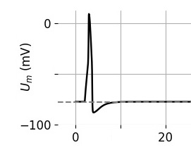
And, we can ask the server to give us a time series of the membrane potential, and that looks like this:



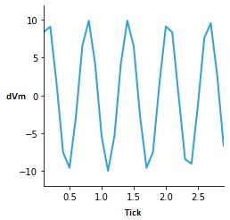
You can see the sin wave generator in action. The neuron never quite made it to threshold, because we kept the input level low. Annie would have complained if we didn't have a synapse, she'd say "You're trying to apply a template to a neuron with no synapses!" Annie watches out for stuff like that. She's very smart (and loquacious when it comes to error messaging). Anyway, that's the interactive process, and it takes about 45 seconds to get through it all (maybe twice that long if you have to think about it). We could have done this with a definition file, it would have taken about as long, it would look something like this:

CELL NAME c EXTENT (1000,1000,0) N_NEURONS 1 ARRANGEMENT GRID_2D
CONNECTION FROM c TO c TYPE INHIBITORY WEIGHT 0.1 TAU 0.05 DIVERGENCE 1
LOAD_TEMPLATE_FILE 'CONES2.TEM'
APPLY TEMPLATE T2 TO CELL c
PROBE TYPE LEVEL OBJECT CELL NAME c FILE 'test_probe.out'
BUILD_NETWORK NAME N
BUILD_SIMULATION NAME S USING NETWORK N
RUN_SIMULATION S TIME 10

The first two lines define the network and the rest is for the simulation. Three lines define the inputs and outputs, the rest is boilerplate. I had to name the cell and the network because they're used in other directives, but the connection and probe can remain nameless. Annie uses defaults for anything that isn't specified, for instance the cell's coordinate center will be (0,0,0) and the template starting coordinates will also be (0,0,0) and it won't move unless you tell it to. In this case template T2 is the same sin wave generator we saw earler, it's set to emit a periodic signal at location (0,0,0) where the neuron is. (We told Annie the cell has 1 neuron arranged on a 2d grid, so she put it exactly in the center of the grid, which is (0,0,0)). In this case everything aligns perfectly and we don't have to make any adjustments to the function. Sometimes when the neurons are in a triangular or hexagonal arrangment one has to give the function generator a little slop so it covers more than just a point. In this case though, our intersections are perfect.

As already mentioned, Annie "applies templates to cells" to create the stimuli that drive an experiment. Templates can be applied to individual neurons too, and even individual synapses, however the most frequent use is to apply a geometric stimulus to a group of neurons within a CELL. In the example retina on the previous page, we had an external stimulus called LIGHT being applied to four groups of photoreceptors called RODS, RED_CONES, GREEN_CONES, and BLUE_CONES. The stimuli we applied were very simple templates consisting of bars, functions, and annuli, and we saw how they can move across the visual field according to a very simple program (MOVEMENT_COORDS, LOOP, REPEAT, and so on). Similarly, we saw how probes can be defined, to examine any part of the network state we're interested in. The rest of the simulation, is trivially easy, you have a Start button, a Stop button, and a Reset button. That's really all there is to it. You can't run a simulation backwards, however you can look at any of the data and scroll through it as you wish, and visualize it in pretty much any form you wish. Annie will generate CSV files that you can directly read into Python as Pandas dataframes, which puts the entire spectrum of data science at your fingertips. Furthermore, any Pandas dataframe can be directly visualized (interactively) in HoloViews, so if Annie won't show you what you want, you can render it in Python with two lines of code. If you prefer R language, many of the same features are available there. Annie gets along with everyone. The only thing she doesn't like is unnecessary complexity, like the connection set algebra where you have to specify your connections with symbols that don't exist anywhere but on APL keyboards. (Are those still around ? I remember buying the special typeballs for my IBM Selectric).

So let's look at some simulation results. Here's an IAF neuron, they're not very exciting, everyone has them. The more interesting part is the sliders on the left, that let you interactively control the parameters of a cell, neuron, connection, or synapse. In most cases you can do this while a simulation is running. There are caveats, for example if you have a variance on your parameters it won't be applied when you use the slider to change things "while" the simulation is running. If you want the variance, you have to stop the simulation, apply the changes, and then start the simulation again. Ticking will stop automatically if you try to change something that would disrupt the network.



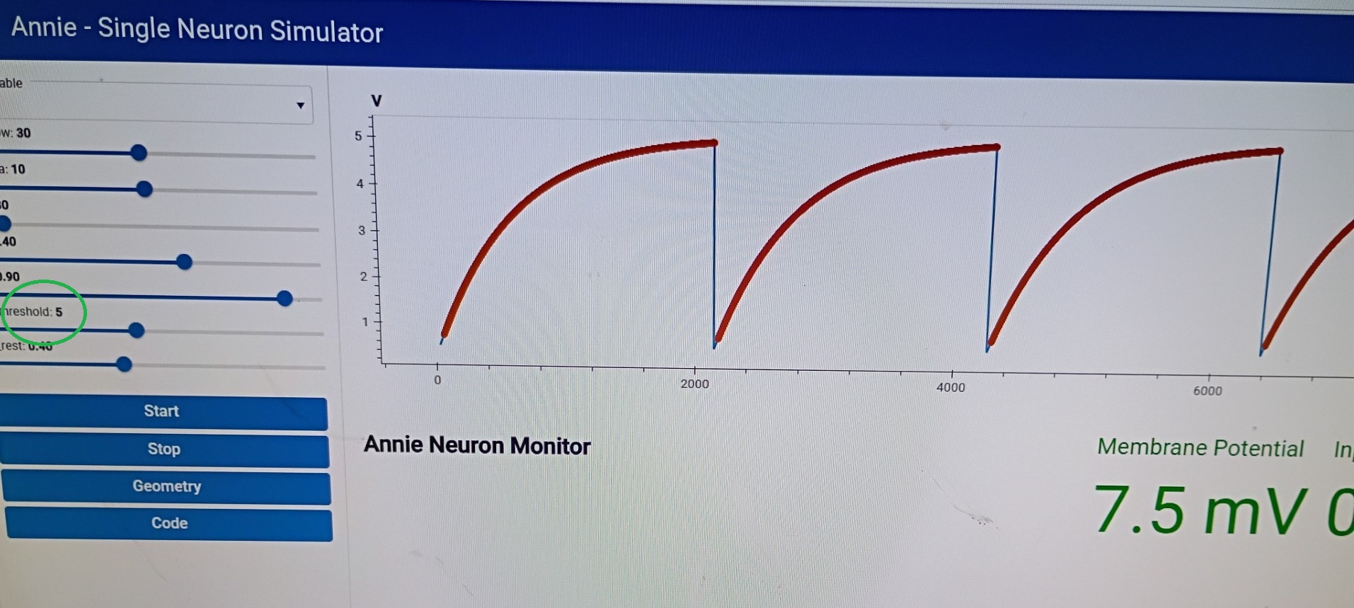
IAF neurons, while boring, are still industry-standard, so we have to include them. Here's a slightly better neuron, this is a version of a Hodgkin-Huxley neuron. And here's where things start getting real, because an H-H membrane starts to get intricate, there are ion channels with multiple subunits and the equations describing them start to get lengthy and complicated. An IAF neuron is parameterized by a "deviation from resting potential", which makes it easy to use Euler's method or any of the Runge-Kutta's to approximate the dynamics. As we start getting into GHK territory these equations start to include powers of subunits and interactions between channels, and thus become harder for the computer to solve. The tradeoff is precision vs speed, and typically when we model a piece of brain we start loosely in favor of speed, and then gradually we wish to become more precise as we zero in on the desired behavior. This is a "workflow", and it stands on the shoulders of giants because people used to do this stuff by hand! Not to mention the genius of people like Hodgkin and Huxley, who somehow decided to try curve-fitting to power functions (and it ended up working). If they'd had Annie it wouldn't have taken them half a year to do the curve fitting, Annie has all manner of linear and nonlinear solvers and they're all accessible with a couple of mouse clicks.



The equations that create this neuron look like something out of Brian2, but you don't have to worry about that (unless you want to, in which case you can). Create a Hodgkin-Huxley neuron this way:

CREATE CELL C NEURON_TYPE HH-3

There are many types to choose from, and you can accept the defaults or further modify your directive if you wish:

      C_M = 1.0             * (uF / cm²)
      G_Na = 120.0       * (mS/cm²)
      G_K = 36.0

and so on.

Here's a neuron with a nice stochastic variance, which was created by altering the Fano factor on a Poisson distribution. This is a common method but it's cheating, in real life the Fano factor is determined biologically. Even the subthreshold noise is voltage dependent (Jacobson et al 2005). Sometimes we're only interested in spike times, and we'd like to know what kinds of information can be carried in a spike train. This question is best answered in the context of the population, because spike trains by themselves mean very little. For example in the hippocampus there are high-frequency spindles in the 200 Hz range and fast gamma in the 100 Hz range, and a typical spike train will include components of both. To decipher such a train one would have to be aware of both the activity of nearby neurons and the condition of local membrane proteins, since sub-threshold membrane oscillations will interact with the synaptic input currents. It gets even more intricate when calcium channels are concentrated "only" in the dendritic tufts and not along the main shafts, or "only" in the basal dendrites and not in the apical. Try as one may, there is no escaping the fact that geometry is central to every piece of a neural network. And quite obviously, the ability of biological system to control their own geometry is central to life.



With Annie, you can work on single neurons as easily as you can work on entire networks. Single neurons are intensely interesting! They can exhibit many kinds of behavior that exceed the integrate-and-fire paradigm. People who like to play with single neurons, are interested in things like ion channel kinetics, and the biophysics of receptor-ligand binding. These are the people who really need the differential equations that Brian2 offers. So, Annie offers them too. Just nicer, and in a way you can visualize. Annie will show you the actual membrane. You can click on an ion channel, and modify its properties. Then run your simulation, and see the results instantly. You can control everything from channel density to modulation by proteins and second messengers. Let's take a look at how this works, using the neuron we created on the previous page. You'll recall we didn't specify anything about the computational aspects of the neuron, we just created its geometry. Now let's look at how we can define the membrane properties of each compartment.

First of all, we'll need a list of the compartments. That's easy, Annie already has it, as we saw on the previous page. And, we don't want to specify each compartment individually, we'd probably like to program some kind of density gradient into the overall distribution of our ion channels. However we need lots of voltage-dependent sodium channels right at the axon hillock, we have to make sure there's a concentration there. How do we do that? The gradient is the easy part, we just add a little more detail to the AXON specification by telling Annie CHANNEL c GRADIENT h FUNCTION LINEAR(a,b) or whatever kind of gradient we want. To get the concentration around the axon hillock, we have to identify the particular compartment we're talking about, and fortunately Annie has anatomical knowledge so you can just tell her HILLOCK CHANNEL c CONCENTRATION 0.01 but if you want it somewhere else you might have to specify a branch point or a compartment ID (which you can easily get graphically by just looking it up in one of the tables - and in general you'll want to name the things you're interested in so you don't have to keep referring to them by their ID numbers - you can name anything and everything, even individual synapses and individual ion channels - even individual branch points on axons and dendrites). Naming came out of the text world, but it turns out to be very helpful for interactive users. Personally, I use a naming convention, that way I always know where to find things. Descriptive naming helps, if your objects are named "a" and "b" chances are you'll run into conflicts and you won't remember what's what. Annie will catch you if you try to assign the same name to two different objects. You can configure her to be case-sensitive or case-insensitive. She won't allow spaces in names, but you can use hyphens, underscores, and periods. Periods are nice, until you get too many of them. Network.nucleus.cell.neuron gets a little confusing unless you use exactly the same format every time. I prefer the descriptive anatomical names like CORTICOSTRIATAL_PATHWAY, and I like upper case because it's easier to read.

Anway, you can tell Annie what kind of mesh you want. If you look at the picture on the bottom of the previous page, you can see that Annie created a compartment at the axon hillock. The compartment wasn't there in the original mesh. The original mesh has no segmentation whatsoever, except at the branch points. So, in its original form, the neuron we created from a picture is unsuitable for the placement of compartments and ion channels, because it has no attachment points. We can segment the mesh in several ways. We can ask Blender to do it for us, or we can ask Annie to do it for us. If we ask Annie she'll assume we want to position channels, so she'll give us a fine mesh with a regular spacing, which we can then ajust. An axon hillock can be loaded up with ion channels in a very simple way, with repeated statements of this form.

NEURON NAME ABC
...
      AXON CYLINDER (1,1,0)
            HILLOCK CHANNEL A CONCENTRATION 0.01
            HILLOCK CHANNEL B CONCENTRATION 0.02
            HILLOCK CHANNEL C CONCENTRATION 0.03

where the channels are defined elsewhere in the file (as they relate, for example, to the parameters in the various types of library neurons). The computational information associated with a channel can be specified at a detailed level, channels can have multiple subunits with varying kinetics, for example there half a dozen different kinds of voltage dependendent sodium conductances, one recent study in the LGN identified 17 conductances important in thalamocortical relay neurons. Mostly to date, channels have been related to membrane resistance and capacitance, but there's a lot more to it. Sub-threshold membrane oscillations are especially interesting insofar as they affect the timing of action potentials, so if we're doing a simulation like the one shown above, we'll be very interested in knowing whether we can affect the population activity in the 200-Hz range by changing a few channels in the nerve membrane. Does the sub-threshold frequency determine the population frequency? Is that why it isn't sensitive to GABA? Answering that question in Brian2 is a nightmare! You have to jump through hoops just to get some authentic basket cell geometry. With Annie... GRID_2D, DIVERGENCE 100, MULTIPLICITY 1000, HILLOCK CHANNEL C, ... that's it, you're ready. You can look at what you have, and then adjust interactively. In simulators like Brian2, inspired by Hodgkin and Huxley, the channel properties are included in the parameters h, m, and so on. Unfortunately there's more to it than that, especially when one has multiple receptor types in the same synapse, and they interact with each other, like AMPA and NMDA receptors in glutamate synapses. Annie has a library of simple kinetics, but if you're serious about your biophysics you're going to need to provide your own interactions, and in that case you're essentially engaging in finite element analysis, which is exactly what you need Annie for. No other tool is going to do this for you, if you don't use Annie you'll have to write your own software, and good luck with that. Even with Claude Code backing you up, it'll take a while. If you're really good you might be able to throw together a one-off, then next time when you need a slightly different geometry you'll have to do it again.

This paper out of Europe is an excellent case study. Listen to this:

"Because human datasets are far from complete, computational models can be used to fill the gaps caused by missing knowledge and propose specific functional hypotheses. Detailed neuron models can be reconstructed from digital morphologies to generate morpho-electrical equivalents, which can subsequently be endowed with cell-specific ionic conductances. Simulations of responses to current injection can then be optimized against electrophysiological recording templates to extract missing information about model-free parameters, such as maximum ionic conductances. In this study, we utilized high-resolution morphological reconstruction of human PCs and unique electrophysiological recordings obtained in acute cerebellar slices from post-surgical cerebellar specimens to generate detailed biophysical models. This allowed us to simulate the electrophysiological response of human PCs under conditions that would otherwise be impractical for the experimental assessment and evaluation of their dendritic complexity and computational capacity".

Sounds great, doesn't it? Right up our alley. Until you start reading about how they did it. In addition to all the complexity up until the point of microscopy (like patch clamp recordings and so on), they traced all the dendritic trees by hand using a Wacom tablet, then they had to use NEURON and BlueBrain to work bottom-up with the ion channels, and they didn't have any human data so they used data from guinea pigs. Then they wanted to look at dendritic spines, so they had to use special software that didn't work quite right and they ended up having to arbitarily correct the Z axis by a factor of about 15%. Next we have this inevitable line buried in the depths of the paper: custom-made Python3/NEURON 8.0 script. The simulator wouldn't do what they wanted so they had to write a custom script. Then at the end of the paper there's a whole list of additional tools that includes MATLAB, native Python, NeuroM, TREES, Vaa3D... you see the problem here. They're in the business of collecting software, like people used to collect vinyl records and DVD's. Fractal analysis of dendrograms has its own tool. Somehow they had to get the data out of one tool and into another, which must have been a special treat. And at the end of the day, what have they learned? The title of the paper is "Human Purkinje cells outperform mouse Purkinje cells in dendritic complexity and computational capacity". Gee, I'm amazed. All that work for this? :)

I'm teasing - and merely pointing out that the ecosystem of tools available to neuroscientists is still stuck in the 90's. Kristof Koch was looking at neural noise on meshes in the 90's. Other people had that idea too, but back then it was supercomputers or nothing. Today, meshes are on the desktop. ParaView is a very popular desktop application for visualizing meshes. Maya can generate animated characters on meshes, complete with rigged skeletons with forward and inverse kinematics. You can make your neurons twitch. Meshes are actually very efficient computationally, the discrete differential geometry is covered very nicely in a series of videos by Prof Keenan Crane from Carnegie-Mellon. One just has to be aware of the mesh storage format, there are perhaps half a dozen in common use and about two dozen more for special purposes. Annie will figure out the format from the file extension or by reading the first few bytes of the file, but for instance there are several varieties of binary STL files and Annie isn't going to try to keep up with proprietary formats. If you're a scientist and you're invested in proprietary formats, you should cut your losses and make the move immediately. OBJ files are perfectly adequate for 3 dimensional solid modeling, whereas dynamic visualizations require the ability to add data to vertices. Annie lets you add arbitrary data to vertices. An EMI mesh requires the calculation of a host of local data including ion concentrations inside and outside the membrane. These are conveniently represented by data structures attached to each point, each face, or each volume.

But wait... there's more. Meshes bring another computationally astounding and visually appealing capability to the table: neural development. I'd like to show you the developmental piece. Axons that grow along pathways, find their targets, sprout and then get pruned. These kinds of simulations are a little harder to put together, because they involve more than just moving templates. So far we've seen that once we have a prototype axon defined at the level of the CELL, we can replicate it down to the level of individual NEURONs by simply telling Annie how much variance to apply to each instance. Some networks will build perfectly this way, while others may require more advanced connectivity. Annie's EMIT, SEEK, SPROUT, and PRUNE directives have time courses and computational rules. We'll get into all that on the next page. It's an entirely different way of combining networks and simulations, if you're used to Perceptrons it can be a bit of a shock. Connections that don't stay put, they move around. Not only that but they change identity, they convert from excitatory to inhibitory and vice versa. And they don't use Hebbian learning, the biochemistry is entirely different. At some point such models become "phenomenological", but it's quite possible to relate them directly to biochemical activity. The phenomenological piece is, you can look at an actual neurite growth cone, there are plenty of videos on YouTube, and understand instantly that simulating it on a mesh would be an intensely complex effort. On the other hand the basics of chemical attraction and repulsion are well understood and in theory it should be possible to model the behavior of filopodia and lamellopodia in something approximating real time.

We'll discuss all these things in more detail, right now most of my time is being spent porting the text-mode application over to the dashboard. When Annie started out she was strictly hierarchical and had several years of detailed error-checking that ensured neurons never existed without cells and that kind of thing. However users don't work that way, they want to go straight to creating neurons, long before they create any networks. So we're doing this right, we've charted out the use cases with UML and we're building the dashboard to accommodate them all. As of this week, you can create a single neuron and use it immediately in a simulation, without having to specify networks, cells, or anything else. You can tell Annie the neuron is a spontaneously active pacemaker and watch its output in the simulator. One couldn't do that a week ago, one had to build a network with nuclei and cells before Annie would start a simulation. Now, you can move neurons into and out of networks on-the-fly. The UML models are needed because some of these things are dangerous, removing error checks is always dangerous, so we needed a detailed up-front map of what to allow and what not to allow. Scientists are very clever people, and they like to push buttons. Annie needs to protect herself against random button-pushing, while at the same time allowing the cleverness that generates results. Porting Annie is a lot of work but it's working and you're looking at the early results. It only gets better from here, the visualizations get richer and Annie gets more outgoing and more reliable. Meshes may seem like a graphical over-achievement in some ways, until one realizes the mesh geometry came out of the supercomputer world, its purpose was to be able to perform nonlinear computations on lattices, the same way we do fluid dynamics. The meshes were originally put in place for computational purposes, not necessarily for beautiful network geometry - it just so happens that in the brain, one can not escape from the geometry, it's an essential part of the networks and the simulations. No one exactly knows what would happen if you flattened out a hippocampus or a section of cerebral cortex. When you section a retina the neurons keep working, but when they're disconnected from their neighbors they work "differently", and sometimes it's hard to say exactly what the difference is, and we need data science and sophisticated network models to help us find out.

The whole purpose of simulation is quantitative elaboration, so we have to spend some time on the details of the math. So far we've seen how a network is built and how a simulation works, and few cheesy graphics with some promises attached to them. It can't be helped, this is a complicated subject. On the next page we'll focus on Annie's METHOD directive, which applies to neurons and synapses, and their parents the cells and connections. Annie knows about all kinds of different neurons. She'll build a network out of Perceptron neurons if you wish, or McCulloch-Pitts neurons, linear neurons, binary neurons, whatever you want. Fitzhugh-Nagumo, Morris-Lecar, Izhikevich, GHK - in many cases, Annie will build the GHK equation for you! You just tell her what kinds of channels are where, and she'll figure out the rest. It comes with the territory, meshes are powerful computational entities (not only can they accept arbitary functions as modifiers, but to compute the finite element one must estimate the channel densities and kinetics, therefore Annie maintains a library of well known channel properties that serve as a usable starting point and can be easily modified with sliders and text widgets). For modern scientific reasons almost every interesting thing Annie does has something to do with differential equations, and the METHOD directive tells her how to update the numbers. The issue with differential equations is they don't always converge. Sometimes they go out to lunch. There are different mathematical methods one can try, Euler's method, Runge-Kutta, in the stochastic world there is Maruyama, and some of these methods will work some of the time, there is no method that works all the time. You can tell at a glance if your differential equations are escaping orbit, suddenly Annie will start complaining about membrane potentials in the range of Volts rather than milli-Volts. Generally, most methods will work most of the time if you're nice with the time constants. When Annie's ticks are in the 0.1-msec range, you can safely use 100-microsecond time constants, but when you try going down to 10 microseconds your equations might start to diverge. You can change the tick time to 1 uSec but then your simulations will take 100 times as long. Sometimes one computational method will work even when another fails. Surprisingly enough, the Euler method often works when Runge-Kutta fails. Sometimes you can use a stochastic method on a non-stochastic problem and it'll make the solution converge. There are no hard and fast rules for what will succeed and what will fail, one just has to be careful when building the simulation. For this reason, it's a good idea to start simple, and make changes incrementally. Debugging a neural network is exactly like debugging a computer program, if you don't have any idea of what the output is supposed to look like you're going to have a hard time. Let's look at the equations, we can learn a lot from them.

In a mesh setting we're mostly dealing with partial differential equations that describe relationships in space and time. These specifically include interactions of the reaction-diffusion variety. This topic merits some discussion, because these terms have carried various meanings over the years. Let's put some context around it. Lately there's been an explosion of neural network models based on dynamic attractors. That word "dynamic" has many meanings. Neurons in networks acquire additional degrees of freedom, they can do things "relative to the population" that they can't do on their own. Phase encoding is an excellent example, and phase encoding implies the existence of a periodic signal somewhere (an "oscillator"). Neural oscillators are subject to entrainment just like pendulums on a bar, and this behavior is described by the Kuramoto model of phase coupling between the oscillators. The difficulty with the Kuramoto model is it's only single-frequency, and it's been solved for some special biphasic cases but in neuroscience the phase-related behavior of subthreshold membrane oscillations is well know and the reality is it can only be described on a mesh. Any other description is nonsensical, because what you have is a bunch of little oscillators at every point in space, and the exact timing of an action potential is going to depend on those oscillators in complex ways. Every functionally coupled pair of voltage-dependent ion channels can form an oscillator. Some of the (few) mesh simulations performed to date indicate that the precise spike timing of a neuron can be influenced by coupling from neighboring neurons. And if you're seeing this in axons you'll see it in dendrites too, you'll get similar behavior in every dendrite that uses calcium mini-spikes, which is probably every pyramidal cell in the cerebral cortex and then some. If, say, I were looking for a way that a neuron might be able to memorize and reproduce a spike train, this would be an excellent place to start looking.

There is some further discussion around this point. Lately there's been a lot of talk about "energy functions", what are variously called cost functions, or error functions, or Hamiltonians or Lagrangians, depending on your discipline. In a nonlinear thermodynamic mesh, the covariances described by coupling functions provide another source of non-local interaction, which in this case is more often deemed to be "regional" rather than "global". In relation to things like dynamic neural attractors, we're interested in what determines the size of the attractor, and its shape. Certainly the network geometry does, but in nonlinear meshes you get standing waves that result from coupling, and in some cases this behavior can be computationally useful. You can do math on a mesh full of oscillators just like you can do it on a Hopfield network, but now you have additional degrees of freedom because of the phase relationships. The point being, that the idea of a "global" variable is still non-biological, there is no such thing known to exist in real brains. What does exist, are "regional" variables, like ion concentrations in the extracellular space, and significantly, the activity in a regionally connected population of astrocytes. It is very likely that dynamic regional boundaries are computationally significant. Some of this is already visible at the level of dynamic attractors, but there's more to it. We need to able to visualize the actual computational boundaries in the simulator. And that is a very tall order unless you have everything on a mesh. Simulators of the Brian2 variety aren't going to show it to you. TensorFlow doesn't come close to any such thing. The computational need is to relate the observed behavior to the information geometry. We're looking at the same thing the biologists look at when they poke electrodes into a live brain - we're looking at spike trains. With the simulator we can see a little more, we can see the local extracellular space too. But on a mesh, we have the keys to the kingdom. We can see everything. We can see exactly how those spikes got created, and where they came from. We can actually visualize a volley of spikes in relation to a traveling theta wave. Without a mesh, that's just about impossible. With a mesh, we get it for free.