Meshing turns 3-dimensional geometry into something computationally useful. And we can have a lot of fun with it! Here's the industry standard Stanford Bunny, and a close-up of the surface mesh.

     

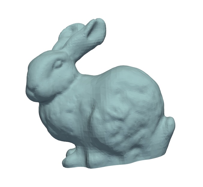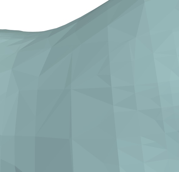
This is "one possible mesh". This can be easily remeshed to any desired resolution. And as we've already seen, a little bit of color goes a long way when it comes to visualization.



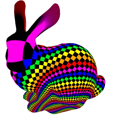
Notice how the mesh algorithm has smoothed away a lot of the detail, especially around the ears. It's given us a nice regular mesh around the body, and if we're studying cardiac vasculature this is good but if we're doing cochlear implants we'll want more detail around the ears. Surprisingly enough, facility with meshes is sometimes hard to accomplish with existing software. There is a community that uses CAD/CAM, another community that focuses on 3-D printing, and yet another community that meshes skeletons with forward and inverse kinematics. The people who do CFD and MHD like gmsh and OpenFoam, and all these toolsets are great for certain things, but they're not exactly neuroscience. Neuroscience has special needs, one of which is scaling, and another involves the maintenance of named objects (like organelles) during the workflow. Believe it or not, as of this writing there is no standard that allows a biologist to accurately mesh the entirety of a single cell. In neuroscience as well as in other medically related fields, large datasets are being aggregated using file systems that came out of the supercomputer world, like HDF5 that underlies the BOSS and MICrONS databases in the AWS cloud. HDF5 is like an entire file system within a single file, it allows the seamless inclusion of enormous collections of diverse file types (like, one could collect DICOM images from MRI, meshes from Annie, and light and serially sectioned electron micrographs, all of the same brain area, all within the same file, organized by metadata). And, the local clients that read these files, don't have to read the whole thing, they can read tiny slices of the data a little bit at a time. For example if we're deriving an SWC file from a series of microscope images, we'll want to keep the source data together with the processed result. And then, we'll want to create a mesh from that, which could be a very large file with millions of data points, and then we'll use that mesh in a simulation, which will create snapshots consisting of millions of data points with multiple computational elements attached to them, at each tick in time. If you're visualizing the simulation results, the most basic need is to be able to scroll back and forth through time, and HDF5 lets you do it one frame at a time so your PC doesn't get overwhelmed.

Another basic need for micro-fluidic simulation is the ability to distribute the computational workload over multiple processors or machines. These simulations can get very computationally intensive, depending on the required resolution. If you need to scale up to the level we're about to discuss, you'll be dealing with several million vertices in each neuron and astrocyte, and you'll have to make some compromises in favor of the calculations - and the compromises you're forced to make are a key determinant of how realistic your simulation becomes. Simple things like an assumption of homogeneity become completely unrealistic when we're talking about 1 nm molecules diffusing through a 10 nm space. If you need that, you have to go to a stochastic simulator and track the path of individual particles. Doing that for millions of data points... well... it takes a while. So typically you'd spin up 50 or 100 machines in the cloud for a few hours, collect your results in an RDS database or an HDF5 file, and post-process them offline as your time permits.

Now that we've jumped through hoops to get a perfect triangular surface mesh, we have more work. Unfortunately, the ugly reality is that if we want to do finite element modeling, we have to thoroughly understand the CAD space, including the file formats, because the finite element tools use CAD geometry. The concept of a mesh is a little different in CAD, a mesh has nodes and elements instead of vertices and triangles. CAD is inherently 3-dimensional, and even though we generated a tetrahedral mesh, it's not yet sufficient. We have to divide our mesh into partitions, so we can stimulate (for example) the tip of a dendrite without stimulating the whole neuron. And, each partition has to be assigned physical properties, for instance if your lipid bilayer membrane has a dielectric constant, or some elasticity or porosity, these things have to be attached to the mesh elements. One can think of the main reason for CAD conversion as "grouping". We need to group our triangles into useful entities. Here is an example of a partitioned neuron, generated from the ANNIE's tool kit:



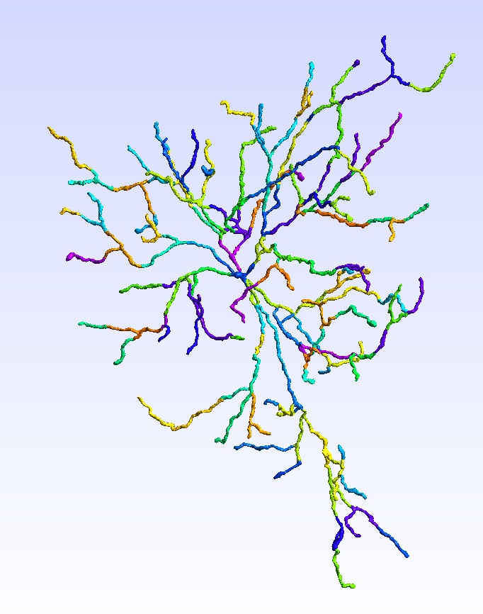
As usual, ANNIE makes this easy for us, and the Annie-Mesh utility is available as a stand-alone tool to bring an original SWC tracing all the way through the OBJ stage and into the final FEM format. Without Annie, we'd have to use a mixture of tools like gmsh, FreeCAD, Salome, and several others, to get our mesh into a useful form. (There are commercial tools available that will do the job, if you prefer to pay, but they're not necessarily any easier or faster). With Annie-Mesh you just load your SWC, then push the buttons on the left hand side in order. (They're split up just in case there are any errors along the way, for instance if you have self-intersecting branches Annie will let you know). Ultimately we'd like our mesh in .msh form because it's an industry standard and it's portable across various FEM engines. Unfortunately there are versioning issues in the mix, some of the older software won't read the newer formats. As long as you stay within Annie you're good, if you have to go to MOOSE you'll probably need to get your mesh into some other format. Remember, Annie has the biological materials, and MOOSE doesn't (yet). If you need to know the details of .msh files, this obscure gem has hidden within it the keys to the kingdom, and it's practically the only place that does. Check out Section 4.

Once you've created an acceptable geometry with your mesh, you can import it into a CAD engine and see if it works. Elmer-GUI is super-cool for this purpose, if you can read your mesh this way you're good to go. You'll want to double-click on the tip of a dendrite and make sure it turns red, if you can do that you're ready to proceed. (Just be patient, once you have a thousand partitions the software slows way down, it might take a second to reflect your changes after you double-click the mouse).



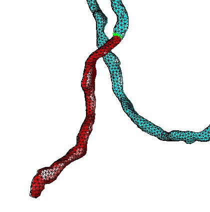
If you can't do this, the mesh won't work. It means there's something wrong with the mesh file. You can debug the mesh file by dragging it back into Annie-Mesh and pushing the Debug button. Annie will check your geometry and reconcile it with your mesh elements and recreate the mesh as needed. In the figure, the little green areas are the boundaries between partitions. These are different from the boundaries "along" partitions, which haven't been defined yet in this pic. When the tip of a dendrite turns red, it's more than just a mesh partition, it's a "physical group" (in CAD language). That means you can assign physical properties to it. You can drag the .msh file into any of the CAD tools that will support this, including the commercial tools. The commercial tools usually have advanced materials that the open-source tools don't have, but it's not hard to create a new material if you need one, you'll have to research the literature to get the material properties and then translate the units as needed. The heads-up about materials is we (for neuroscience) need materials that can change their properties dynamically. For instance you can think about how wood behaves when it gets wet (it saws differently, for one thing) - that's a dynamic change in the material property. Biology has many such dynamic changes.

There is additional work after this, and it may become necessary to revisit this step once the simulation is working, to refine the mesh and adjust the partition sizes. For example, here is the same tracing with much smaller partitions.



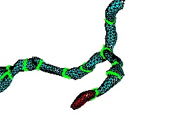
If you stimulate the red piece with a physical force it's very close to simulating a single synapse with a tiny electrode, or sprutzing a little neurotransmitter into the synaptic cleft. Mesh refinement is a different concept, though. Refinement has a specific meaning in the finite element world, it's something you do when your simulation blows up (or ahead of time, if you've been doing this kind of work for a while). Refinement means specifically, you make the compartments smaller near the edges (near the "boundaries", although this term also has specific meaning). In a mesh like the above where the element resolution is in the 10 nm range, refinement may not be necessary. In many cases we'll want to go the other way, to reduce the computational load, we'll want to decimate instead of refine. For instance if we're doing biophysics on an astrocyte leaf, we may only be interested in the leaf itself, and perhaps a nearby branch or two, so the entire rest of of the mesh can be decimated and the number of active nodes reduced from 10,000 to a few hundred. However in refinement, we want to make the mesh more resolute, so the estimates of 'dF' become more precise. This is an example of mesh refinement, you can see how the cells get smaller near the edges.



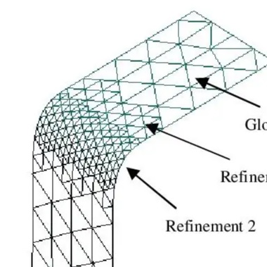
Refinement is sometimes a good idea (or becomes necessary) near corners and sharp edges, and around discontinuities and areas of high curvature (holes, organelles). Eight times out of ten unless you've very lucky, a simulation will blow up the first few times it's tried, and usually there are specific areas in the mesh that can be identified as problematic. These areas become candidates for refinement. There is a phenomenon called "locking" that plagues discrete simulations, and it's worth understanding in detail (fast forward to the 28 minute mark if you wish). Locking can sometimes be addressed by changing the computational method, but usually it requires some modifications to the mesh. In many kinds of FEM, there are boundary equations coupled into the nonlinear core, and near the boundaries the numbers get small and the computational engine has a harder time. You'll hear the term "stiffness" a lot, it has to do with the matrix M we talked about earlier. When the matrix is well behaved (like, invertible), it's easy to solve, but most FEM simulations aren't particularly well behaved, especially around the boundaries. The issue raised in the video is fundamentally one of scale. The size of the mesh elements matters. When they talk about "bulk modulus" they could be talking about a piece of wood, but they could also be talking about a biological membrane, or a piece of the cytoskeleton. There are other reasons to pay attention to mesh scale, for instance if there's an oscillatory stimulus the mesh elements have to be considerably smaller than a wavelength, that kind of thing. (In biology we won't have such problems till we get up into the microwaves, which is beyond the scope of this discussion)

The next step after meshing, is putting the bunny in a cage. Or alternatively, putting the brain in a sphere. Or equivalently, bringing two neurons so close to each other that they practically touch (20 nm, just like in a real brain). Why are these things similar? Because they all deal with fields, and boundaries. Before applying any electric currents, we need to define the properties of our materials. Materials are substances with physical properties. In a solid body model your material might be aluminum, or wood, but in biology it's going to be a membrane or a piece of cytoskeleton. Since we're not doing molecular dynamics (yet), the channel composition of a patch of membrane has to be represented statistically, and thus different materials will have different average properties. This will work for us as long as averaging makes sense. You "have to" partition your mesh into at least as many compartments as you have differences in properties. In practice this means you're going to group vertices and faces together, in such a way that they form computational compartments. It seems like we're inverting all the hard work we did to get a smooth mesh, is there a faster way we could have retained the original skeletal compartments? The short answer is... no. We needed the smooth mesh to be able to triangulate it, and now all we're doing is grouping triangles. Let's look at why we'd want to do this. Here why:



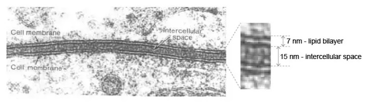
These membranes less than 20 nm apart. The membranes themselves are about 7 nm thick, each. This situation is the exact opposite of an EMI model, where both intra- and extra-cellular spaces are modeled as infinite isotropic and homogeneous domains. Reality demands that we calculate the field effects along every point in the 20 nm space the separates the two membranes, because this is the only place that calcium ions can diffuse. Calcium ions diffuse in the extracellular fluid, and they're also charged particles that respond to fields, and they also bind with other molecules and result in the generation of mechanical forces in the cytoskeleton. We have no choice but to do multi-physics in this tiny 20 nm space. Certainly this qualifies as micro-fluidics, since we have vesicles ejecting neurotransmitter into the space, and gently pulsing CSF and blood flow that sends tiny pressure waves through it. One thing we'd like to do, is stimulate the synapse so it releases a few vesicles, and then observe the activity on the postsynaptic side. If this were a traditional simulation, it would be easy, we'd just attach an external node to the object we want to stimulate and put a probe on the object we'd like to observe. However here, we have to apply a physical condition to a patch of membrane, so we have to distinguish this patch of membrane from all the other patches. If we stimulate a single triangle we're basically affecting one or a few ion channels, so the logical thing to do is group a few triangles into a special patch that we can conveniently stimulate by applying a physical force to it. The result is shown on the next page.

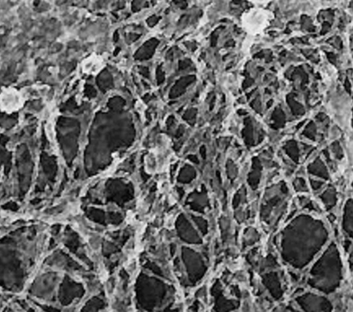
The next step after meshing is scaffolding, which is a universal technique but takes an idiosyncratic form in neuroscience. Scaffolding includes things like putting a cytoskeleton directly underneath your cell membrane, or placing organelles inside the volume of your cell, or attaching things to other things, like maybe some cell adhesions proteins that sit in the tiny gap between a neuron and an astrocyte. For instance, the picture on the home pages shows endoplasmic reticulum inside an astrocyte. How did it get there? How did we do that? It looks different from the regular geometry of a structured cylinder. The important part is that the ER saccules don't just float around, they're actually attached to the cell membrane. The resolution of the image on the home page isn't quite good enough to show the attachment points, for that we'd have to increase the precision of the visualization. (Which we can do, for molecular dynamics and other purposes). Mitochondria are another example, they don't just float around inside the cell, they're attached to the ER. Building the skeleton of a cell is important, especially for the multi-physical aspects of the simulation. Internal structures are obstacles for fluid dynamics, and they may change shape and move around mechanically. Scaffolding often makes the difference between a working biophysical model and a toy. Here is an electron micrograph of a real cytoskeleton. You can clearly see the actin scaffolding, and there are many examples of such geometry in nature (a cross section of a blade of grass reveals "percolation", and we can use biophysical models to determine whether the same phenomenon occurs in the cytoskeleton).



There's more to scaffolding than just building the cytoskeleton. Scaffolding has a specific meaning in the FEM world, insofar as it assigns different materials to different parts of the mesh. For example, how are we going to stimulate a beautifully meshed neuron? We have two choices, we can try to put an electrode somewhere, or we can virtually open up a few ion channels with the timely application of forces. We'll choose the latter method for now, because electrodes are complicated in FEM simulations. To get started, we can carve out a tiny portion of the branching tree, and assign a different conductivity to it, which in the FEM world equates with a different material. A "material" encompasses the biophysics of a patch of membrane, so if you want your channels to open and close in real time, it means you have to alter the properties of the material in real time. This is certainly not the preferred way of handling things, but it makes the simulation work at an early stage of the workflow. To do this we first carve out a tiny piece of the tip of a dendrite, and assign a special high conductivity material to it. Then, we set the initial conditions so this compartment is the subject of a force. In the language of neuroscience, this is equivalent to applying a steady current to the membrane patch. This will hopefully be enough to raise a working simulation and observe the result of the input current on the equilibrium conditions. To do this with a FEM simulator, we have to translate all our interventions into physical forces. We'll either have an electromotive force, a mechanical force, or some kind of local coupling like reaction-diffusion (maybe we're doing optical uncaging or something).

Attempting this workflow repeatedly and in volume, quickly raises other issues. To open a calcium channel, we have to apply a force to it (like, a trans-membrane voltage), and that means we have to isolate the channel, we have to be able to identify it so the simulator will know which channel to apply the force to. The industry-standard way of accomplishing this is "named objects", and the concept applies across the board to all the objects we might encounter in a simulation. If this were a molecular dynamics simulation we could name a molecule, and then watch Mollie as she moves through the membrane. Generally speaking, in the final mesh file there will be all manner of objects - there will be organelles, and molecules, and virtual groups we just want to average over. It would be nice if the name of an object were human-readable, but it could also be just a unique number, the latter condition is usually found because it reduces the memory footprint. In GPU simulations the identifiers can be passed as arrays while the strings are left on the CPU side. The simulator doesn't care about names, it just needs the numbers. They become additional data items attached to mesh elements along with the physics. Identifiers single out objects in the mesh, and groupers group them together.

So let's keep talking about shape. How does the shape of a calcium puff around a tiny piece of endoplasmic reticulum relate to the shape of a dynamic neural field or the shape of an energy surface in a Hopfield network? To answer these questions, one must realize that high resolution computational meshes are absolutely essential, we can't answer these questions without them. In the past, scientists have been forced to use small low-resolution models unless they had access to supercomputers, but today we have a reasonable chance of approaching these answers with commonly available toolsets. Along with that understanding though, comes the realization that familiarity with the cloud is essential for this effort (and for neuroscience in general), and some knowledge of AI helps too, and these are still steep learning curves for people whose world is ordinarily wetware and microscopes. Annie wants to help bridge that gap by making computational modeling easy. Easier than NEURON, easier than TensorFlow, easier than VTK. We've seen the general landscape on the last few pages, let's digress for a moment and talk about why we're doing this. What good is it, why does it mean more than just solving a Nernst equation? The next step after generating a suitable computational structure, is deciding what to do with it. Let's take a little detour, and consider the mesh-building we've been doing on the previous page, in an entirely different context. Let's begin with a visual system that has the well known architecture consisting of some orientation and ocular dominance columns. We can generate such a network with amazing ease using Annie, as we've already seen. Have a look at these slides from one of Shun-Ichi Amari's talks on information geometry.

     

     

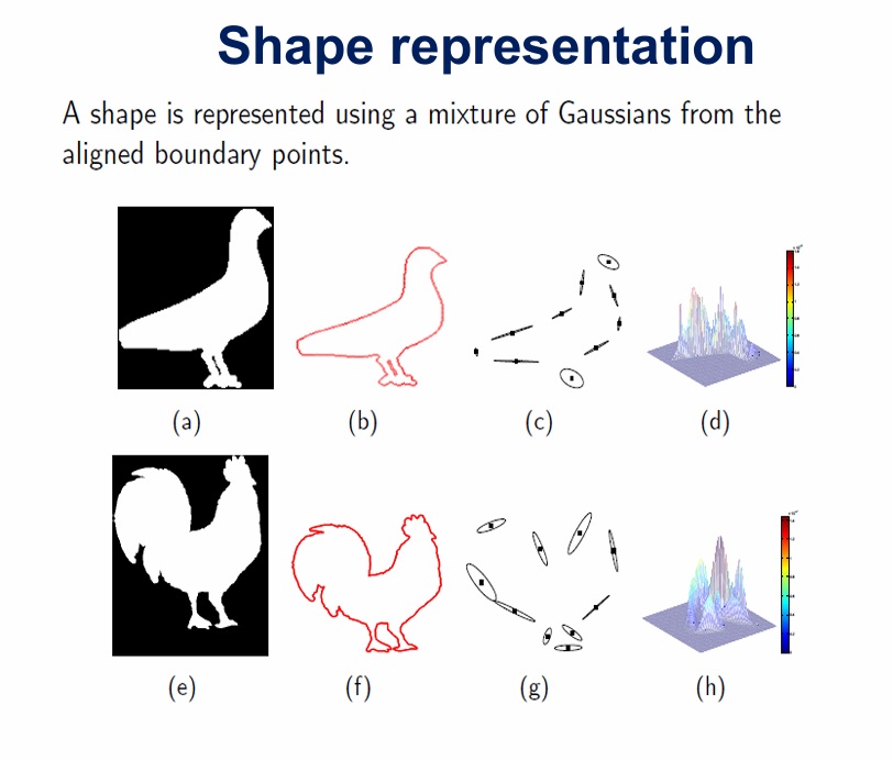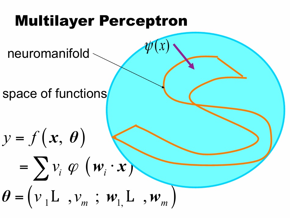
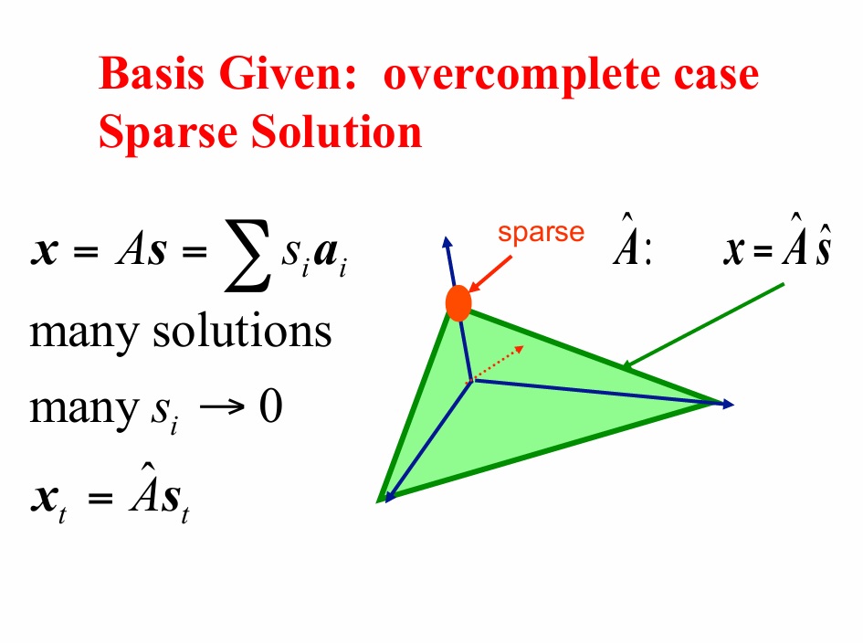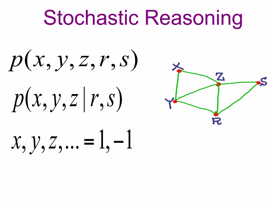
The first image shows some shape analysis, that starts from a slightly different view of what exactly constitutes a receptive field. The interpretation shown here is similar to the one proposed in the theory of dynamic neural fields. The idea is that things like orientation can be parameterized locally in terms of basis functions that are essentially differential operators. The second image shows a manifold of such operators being activated as a range of possible solutions to a set of inputs. The third image shows the division of the manifold into computational cells, and the fourth image is a computational mesh - one that takes us from shape, to reasoning about shape.

This is an abstract example, but it illustrates the many possible relationships between spike trains and mesh structure. One can calculate electric fields on a mesh, as easily as one can calculate ion concentrations. The geometry of a mesh is such that physical relationships can be determined by circulating around loops. The fundamental theorem of calculus tells us that integrating a differential form is equivalent to taking the value of the function at the beginning and end of a path. In three dimensions, Stokes' Theorem tells us the same thing - what happens inside the volume is reflected at the boundary. In this regard, the geometry of the information stored in a neural network is not so far away from the shape of a bunny, it just has more dimensions (and the basis functions might look a little different). Take a look at the first image above - the basis functions in this case are conjectured to be small Gaussian shapes related to local orientation columns. More generally, any shape (including shapes implicit in point clouds) can be precisely represented as a combination of basis functions, in exactly the same way that we represent meshes as linear combinations of basis functions. There is evidence for precisely such a set of parameterized coordinate systems in the entorhinal cortex and the circuitry around the hippocampus - the exact circuitry where the place cells, grid cells, boundary cells, and time cells are found. The time cells look like they're arranged in exactly the manner that Dr. Amari is proposing, there is a range of ramping that provides a set of basis functions. The direct applicability of the mesh to the Kullback-Leibler geometry is an amazing coincidence that requires thorough exploration. There's an interesting glitch in this story though - STDP (spike timing dependent plasticity) requires functional astrocytes. It doesn't occur without them.

One should take a moment to consider the significance of this observation, because it reconciles two disparate and seemingly conflicting results. The time course of STDP is just a few msec in either direction of 0. However the calcium waves observed in astrocytes are slow, mostly they're in the range of seconds rather than milli-seconds, although a small of fraction of the astrocytes seem to be faster. But this latter observation is made by calcium imaging, which focuses on the cell body. It's almost impossible to see what's actually happening in an astrocyte leaflet. The connection with STDP indicates it must be very fast, on the order of a few msec - much faster than the changes in calcium concentration that occur in the interior of the cell. This situation is actually depicted in the animated image on the previous page, one can see that the calcium micro-domains move more slowly than the changes in the normals at the boundary of the mesh. The difference between reality and the depicted simulation, is that the boundary of an astrocyte isn't a planar edge. In fact it looks more like the dendrite of a Purkinje cell. Which means those changing boundary conditions are going to take on a detailed and complex shape. Which means, so will the micro-domains. Hmm...

There is of course a contrary hypothesis as well, which is that the astrocytes merely regulate the extracellular calcium, and it is that which is required for STDP. How to test this? We could go down a rabbit hole talking about how people actually generate STDP, but we won't. The goal is to visualize the shape of the interaction between the astrocyte and the neuron. To predict how the neuron will behave, there is no other solution but a computational mesh. The scale of the connection is too fine to treat the neuron as an entity, and an astrocyte can contact a million neurons and ten times that many synapses. And we haven't even touched on all the issues around glutamate, like multiple receptors with different time courses, spillover and (re)-uptake, ... the list goes on. Anything less than a computational mesh is going to abstract all this stuff away. We could be completely brutal and say it another way: machine learning has shown us beyond any shadow of a doubt that two-dimensional sheets of Hodgkin-Huxley neurons are inadequate. (Neuroscience already knows this! But some of us seem to be having a hard time letting go of the old ideas). In the hippocampus, even the careful placement of ion channels is inadequate, so far there is no combination of channel geometry that replicates the full spectrum of neuron behavior. And part of that is we don't know what the astrocytes are doing. They're needed for learning, and they're also involved in Alzheimer's, and we know a little bit about the chemistry of IP3, but we're still limited by technology because calcium imaging of actual geometry still requires registration. The resolution isn't good enough to visualize an astrocyte leaflet in action. This is an area where simulators can provide a value-add, by making predictions at levels that can't be easily visualized, and translating them into results that can.

The precise positioning of IP3 receptors in the ER membrane is biophysical, and to the extent we can prove things like laminar flow and laminar charge, one is led to question whether these factors influence receptor placement and the shape of the cytoskeleton. One thing we already know, is that astrocytes can adjust the timing window of STDP, and in the neural network as a whole this is a complex interaction, because astrocytes also respond to GABA from inhibitory interneurons, and a range of other neurotransmitters and neuromodulators. In turn, astrocytes emit gliotransmitters and regulate local calcium and proton concentrations, and every evidence we have says this occurs at the level of individual synapses, it's pathway specific and cell-type specific. Another thing we know about astrocytes (and dendritic spines as well), is they're highly motile. They move around, and they adjust themselves as the size of nearby structures changes. One is therefore led to ask whether the motility is related to factors like charge. The physics of biological charge at a microscopic level is fascinating, the Debye layer around a charged membrane is maybe 20 nm which in many cases is about the same as the distance between a neuron and an astrocyte. The electric field across a neuron or astrocyte membrane is enormous, it could be tens or hundreds of millions of volts per meter (in some cases it's very close to the dielectric breakdown of a lipid bilayer!). Then we have the issue of sub-threshold membrane oscillations, which appear to be nearly ubiquitous in cortical neurons, and since spike timing matters and it's known to be mutually modulated by ongoing oscillations, we're led to ask whether the spatial pattern of calcium puffs directly determines the local pattern of phase relationships. If that's true, then calcium micro-domains equate with computational domains, and shape matters. This hypothesis takes us directly into Shun-Ichi Amari's world of information geometry, where the shape of information is related to Riemannian manifolds that are computable in the same way we compute meshes.

Earlier we mentioned dynamic neural fields. When we're talking about a mesh, we're essentially trying to discretize continuous geometry. We do this because the closed form continuous equations are too hard for the computer to solve - it can be done, but it takes forever. Machine learning also looks at neural networks in a discrete way, and the discrete view gets implicit representation in a plethora of neuroscientific concepts. With dynamic neural fields, we go the other way, we build a continuum approximation from discrete geometry. In both cases, the idea is the same, they're just different ways of handling the concept of "d"x (and in discrete time simulations we also have to deal with "d"t). We've already seen how the exterior calculus provides a computationally useful way of linking the two perspectives. However, there's another rub, another angle entirely. It relates to the dynamics of both discrete and continuous networks.

Traditionally, the machine learning view has considered neurons as discrete entities, and connections between neurons as discrete isolated entities. This leads to an algebraic representation that's very powerful, it's the foundation of modern AI. But an interesting thing happens in real brains. In a network where there are many, many, connection "circuits" with different physical and geometric extents, the solutions of both discrete and continuous equations predict the existence of solution "modes" that reflect themselves in the power spectra of regional activity. One can imagine for example, a guitar string in one dimension, or a drum head in two dimensions. In the continuous geometry, the "wave modes" result in the sounds we hear, and there are "overtones" that are harmonics, multiples of some primary mode. However in these musical instruments, the boundary conditions are fixed - and indeed, when one looks at a neural network from a connectionist standpoint one can easily be absorbed into the anatomical subdivisions (which are indeed real, they reflect genetic, morphological, and functional groupings). But here's the rub - in very large networks, one can use Annie to shape the large-scale geometry, a concept that was shown on the About page and several other pages. In other words, one can take a square sheet or 3-d volume of neurons, and re-shape it so it matches the geometry of a real brain, like, the curves of the cerebral cortex and the sulci and gyri of the surface. One can then compare the dynamics expected from local interactions (like, computations within a cerebral column), to the dynamics of network-wide interactions (of the type one might see in an fMRI, for instance the default mode network). It turns out, that the spectral dynamics of the human cerebral cortex concentrate in the first 100 modes, that is, they're long-range, not short-range. Spectral measurements indicate wavelengths on the order of 4 cm, which is approximately a third of the brain, and the key feature of these spectra is they match the actual geometry, not the connectionist geometry.

What does that mean? Well, it certainly tells us shape is important (and we already knew that). The mapping of connectionist pathways into actual brain geometry is somewhat troubling from a computational standpoint. If the connectionist mapping were the only thing going on, there would be no such favoritism in the long range modes. The spectral observations suggest there's some kind of geometric "coupling" between diverse connection pathways. And, in a way, the idea of dynamic neural fields is an extension of volume conductor theory, where the brain is considered as a big sphere and EEG signals are interpreted in terms of currents within the sphere. How does this make sense physically? Well, the low hanging fruit is the idea of electrical coupling between synaptically unconnected neurons. And indeed, the influence of external electric fields on the brain is well documented, and it's used every day in treatments like deep brain stimulation. Another avenue is the presence of astrocytes, which control extracellular potassium concentrations and communicate regionally in a way that links the nano scale to the micro and mm scale. In either case, we would like to quantify how significant this effect can be, in other words in a given network, how much weight should we assign to the discrete geometry and how much to the continuous geometry?

If one were to look for a "nearly continuous" aspect of network construction, one would probably focus on the smallest structures we know of in the neural network - the dendritic spines. It turns out, that the tufts of apical dendrites have very different computational properties from the rest of the neuron, they have different channels with different time courses and emit dendritic spikes related to calcium, as well as NMDA spikes and other interesting behaviors. These computations are very local, the dendritic spikes don't propagate very far - so if one were looking for a minimal computational unit in the brain, this would probably be it. The complexity arises when one considers that this entire finely meshed dendritic network with discrete connection points, is embedded into a physically continuous syncytium provided by the astrocytes. The astrocytes wrap 80% of the synapses in any given brain region, and there are other astrocytes that contact the nodes of Ranvier in myelinated axons leaving the cortex. This provides ONE way of linking the discrete and continuous views - embedding the entire connectionist network into a continuous syncytium. There is another way to link these views, and that is the statistical approach promoted by information geometry. In this view, discrete operations are performed on a manifold, in much the same way we build meshes from surfaces. Just like in our biophysical modeling, most of the time we don't need the whole manifold, we only need a small part of it. And, just like our meshing efforts, increasing local resolution is a way of "paying attention to" a small part of the mesh.

The most interesting (and useful) part of this, is there's a direct relationship between the algebra and the geometry. But what about the dynamics? How do oscillations in neural networks play into this picture? Well, in multi-state neural circuits oscillations usually represent a more highly driven state than simple integration. Typically a neuron will fire in response to simulation, and as the simulation gets more intense the neuron will begin to burst (oscillate). The Kuramoto model suggests that oscillations of the same frequency, that occur at different locations in the brain, will eventually begin to phase-align, and phase alignment results in a high degree of covariance which in turn is reflected in the power spectrum. Oscillations give us a context for understanding spike timing. In neurophysiology there is the concept of TTFS ("time to first spike"), which means the interval between when you apply the stimulus and when the neuron first responds. But this concept assumes we know when the stimulus occurred! In a real brain we don't, except insofar as we can synchronize the population behavior of neurons, which generally occurs well after the first spike. But in an oscillatory environment we can have "phase encoding", which is just the relative timing of spikes and field potentials. Phase encoding sets up geometric patterns in the network, and to the extent the oscillations can be made smooth or "nearly continuous" we have a nice natural way of linking distant brain regions.

To get a neural network to behave this way, requires pretty careful tuning of the network parameters. And, it requires us to scale in our thought process, over all 8 orders of magnitude between nm and cm. We have to balance excitation and inhibition across the network in such a way that the long range connections remain nicely behaved, and we also have to satisfy the connectionist requirements for visual processing, and we also have to describe the processes underlying synaptic modification, and finally we have the biophysics of ion regulation at the tripartite synapse, and the concepts of electrical syncytia and the influence from external electric and magnetic fields. "Multi-physics" is a pretty good way of describing this situation, isn't it?

If you're still asking "what does this have to do with fluid flow and charged particles", we can return for a moment to the idea of diffusion in a space that's only 50 nm wide, shaped in odd ways so it wraps around synapses and spines, and filled with charged particles like calcium ions and all manner of receptors, channels, and modulators. The membrane potential of an astrocyte is around -85 mV, slightly more negative than most neurons because of a high potassium permeability. At 10^7-10^8 V/m, with a Debye field of 20 nm in any direction away from a membrane, there is a favorable channel only 10 nm wide through which hydrated ions need to diffuse. A hydrated ion could be a quarter to a third of a nm, and glutamate at 0.8 nm is a large molecule in that context. Each is electrically polar, and water is paramagnetic. In this situation one expects the flow outside the leaflet to be greater than the flow inside. This is one of the most basic things we can verify with a simulation. We can also look at the equilibrium conditions quite easily, and that helps us understand whether our geometry is correct. We can adjust the mesh size so it's larger than the small molecules, that way we can use a statistical approximation over patches of the membrane surface. We can also run Monte Carlo simulations and track the path of individual stochastic molecules. That's an interesting exercise because it's still very hard for digital computers to create random numbers - although there are now photonic devices that can do 300 million per second without engaging the CPU. Anyway, we're interested in the generation of calcium puffs, which have shape that's related to the shape of the endoplasmic reticulum combined with the distribution of calcium ions. These tiny little puffs combine in an as-yet-unknown way, to create heirarchical calcium events in astrocyte networks, that can propagate over long distances and affect millions of synapses at once. The impact of such an effect includes computationally significant phenomena like the modification of regional energy functions. If any cell in the brain's networks is capable of calculating a regional energy function, astrocytes are in one of the best positions to do so. They tile the brain into mutually exclusive regions, each astrocyte might contact 100,000 neurons (at 100 neurons per mini-column that would be about 1000 processing columns). The local concentration of calcium directly affects the release of all manner of ions, gliotransmitters, nutrients, and other molecules from the astrocyte into individual synapses. It is thus inevitable that shape matters, because the synapses are so close together they require spiny extrusions to keep them separate. We're specifically interested in the ability of astrocytes to impact the timing of synaptic events. We already know this happens in learning paradigms, at time scales slightly longer than the EPSPs themselves. It is highly likely that there is influence at other time scales as well, both faster and slower than STDP. The classical equations like Nernst, H-H, GHK, Poisson, all point to the importance of charge regulation, and ultimately a mesh becomes the best place to reconcile the ideas of ionic "concentrations" (which is a statistical concept), with the idea of the probability of an ion moving through a channel that happens to be open at the same time (which is a stochastic concept). To really find out what's happening with these astrocyte leaflets, we need to do both. One of the great things about this approach, is a negative answer is as good as a positive one. If we can definitively say "this is not the way it works", we've learned something. If one model works but the other doesn't, we can find out why, and refine the models accordingly. If both models work and give us the same answer, chances are good our representation is accurate.

On the earlier pages we showed a particular form of topological mesh, that's well suited to geometric computation, using discrete differential geometry and the exterior calculus. In this representation, it doesn't much matter what the actual shapes are, as long as they're computable. Triangles work because they're easy to orient and there are plenty of algorithms to make them efficient. The "other" way of looking at fluids, as a stochastic set of movements and collisions, is known as the Boltzmann Lattice (or Lattice Boltzmann) Method. This method is more complex to implement when the assumption of isotropy breaks down. The method is friendlier to regularly structured square lattices, of the kind shown at the top of the About page. However we can use the methods of information geometry to reframe the cells in terms of Kullback-Leibler divergences on a Riemannian manifold, and thus retain the simplicitly of triangular organization. (This is a bleeding edge concept, and at this moment Annie will get you about halfway there, no problem setting up a square lattice if you'd like to try it the old fashioned way, but calculating KL on a random triangular mesh is computationally intensive and nowhere near as fast as incompressible Navier-Stokes on the same mesh). As usual, it's the assumptions that matter. If the reason to use LBM is that the continuum assumption is breaking down, then it also makes sense that isotropy would break down too. The concept of the "average statistical distribution" of particles and their properties becomes a set of tensors that can't be easily looked up in a table. It's a lot harder to introduce shape into a Brownian situation than it is to apply it as a well known geometry. Nevertheless, Annie will build a square lattice for you and you can attach whatever functions you want to it, and if you choose to pursue this path you'll hit the boundaries of a bleeding edge very quickly, and in that case Annie is open source and welcomes your contributions!

We started with Annie as a traditional simulator, then talked about ion channels and membranes, and now we're talking about information geometry. Annie makes no distinction between membranes and populations, they're all part of the same big computational mesh. This is what allows Annie (and you) to visualize things like the phase relationships of spiking neurons in the hippocampus. I encourage Annie's students to engage with the sample workflows and actually build a real neuron from ion channels, to see what's involved. A hippocampal CA1 neuron is an excellent case study. The concentration of sodium receptors in the axon initial segment is 50 times higher than it is in the rest of the neuron, and the initial segment isn't directly attached to the cell body, it's distal by a few microns (as determined by the location of the ankyrin-G protein). When this neuron fires, the action potential travels down the axon in the usual way, but it also travels backwards up the dendritic tree, because this neuron is a little different from L5 pyramids and it's missing an inwardly rectifying potassium channel that normally prevents such antidromic invasion. When the action potential reaches the dendrites it triggers calcium influx in the apical tufts, which increases in the presence of depolarization (there is a sodium-calcium exchange current that plays into this, that ends up being important for STDP - which in turns provides a suggestive link to the astrocytic effect on the same process). These neurons have thousands of dendritic spines, each of which is capable of generating its own miniature action potentials. Each little patch of dendrite is like its own little neuron, you can basically stuff an entire convolutional network into a single neuron this way. These neurons are multi-stable (a capability endowed by the configuration of ion channels), they exhibit plateau potentials related to an "up" state during which their behavior is considerably different from the "down" state. In the context of a population theta rhythm, there are multiple sophisticated calculations that take place before the neuron ever fires an action potential. The calculations are heavily dependent on local calcium micro-concentrations, that affect the presence and timing of dendritic mini-spikes. Research has already shown that the timing of action potentials and synaptic events can be affected by both astrocyte chemistry and extracellular fields. Therefore, to study such a population of neurons, one needs to able to theoretically link the activities at these different levels, and move seamelessly between the levels to visualize them at any needed level of resolution. Visualizing a mouse brain is only the beginning. Annie is here to help take us to the next level.

Here is some food for thought. Let's do a thought experiment. Let's say, we have two neurons, A and B, and they each have a refractory period of 1 msec. The question is, what is the smallest interval of time these two neurons can discriminate? Well... we get the best resolution if we stagger the spikes. For example if neuron A is firing at 100 Hz, we can make neuron B fire at the same rate but 180 degrees out of phase, and that way the interval between spikes becomes τ/2, and we can discriminate this interval based on which neuron is firing, or whether they're both firing or not firing. If we increase the number of neurons from 2 to 3, then we can resolve τ/3, and for N neurons we can resolve τ/N this way. This is more or less the mechanism used in the auditory system of owls and bats, to get sub-microsecond resolution from neurons with much larger refractory periods. Consider then, what happens in a cerebral cortex where we have 10 billion neurons. Let's be realistic and pare that number down, and consider that a cerebral processing unit might equate with a column, so say 100 neurons or so. What kinds of time intervals can 100 million processing columns resolve? If we're being old-fashioned we could abstract the output of a processing column as a single number, like for instance the rate of firing of a layer V pyramidal cell. If we imagine this single output has a similar refractory period and we apply the formula, we get 1 msec / 10^8, which is a few picoseconds. To understand this in context, consider how long it takes an electromagnetic field traveling at the speed of light, to get from one end of the brain to the other. We have a 15 cm brain, at 3x10^10 cm/sec, gives us a fraction of a nanosecond. Hm. It appears we have a couple of orders of magnitude headroom. So how many ensembles could we put together, to make the resolution approximately equal? Well, looks like somewhere between 100 and 1000, as a general swag. How interesting! How could these ensembles be organized? We already know neurons engage in every one of the traditional forms of modulation, amplitude, frequency, phase... and they do frequency modulation at multiple levels, part of which involves an elaborate control system with up states and down states. They do it by themselves, and they do it in populations. Gee, that doesn't sound very much like a McCulloch-Pitts neuron, does it? Heck, it doesn't even sound like a Hodgkin-Huxley neuron! It sounds like a very, very smart neuron. One that gets even smarter in populations. One perhaps, that when assisted by astrocytes, can resolve spatial manifolds down to the level of tiny little calcium puffs in astrocyte leaflets. If the shape of an astrocytic domain determines the effectiveness of a synapse, we have a direct link between biophysics and information geometry, which in a way, is the holy grail of both neuroscience and machine learning. Such a relationship would allow us to model and calculate the information content of sharp wave ripples in the hippocampus, which are known to be computationally and behaviorally significant.

One can generate intricate dynamics with traditional simulators. For example the NEURON, Brian2, and Nest simulators combined with equations that describe channel behavior can generate all manner of interesting dynamics, at the single-neuron as well as population levels. All three of these simulators allow computational compartments, for example one can break up an axon or dendrite into multiple cylinders and apply a cable model. But there is a level beyond which these views can not go, because the computational structures inside these simulators are not meshes, they're not suitable for spatial multi-physics. They come close, in many ways, and for some purposes the approximations inherent in these traditional approaches are perfectly adequate. However the scaling of these approaches is cumbersome. To test a theory like the above, one has to scale from micro-fluidics to populations of millions of neurons, let's say over a range from about 1 nm to about 10 cm. To fully appreciate the difficulty of scaling over such a large range, one has only to realize that in real life, we require electron microscopes to get down to the 10 nm range. In real life, it's practically impossible to visualize an astrocyte leaflet, typically the resolution of 2-photon calcium imaging isn't good enough to give us the details. We can look at leaflets with an electron microscope, but that isn't going to show us the calcium puffs. To bring those two things together, is a challenge! To visualize the shape of a puff, might even be a pipe dream. However a good simulator can calculate the physics for us. And with the physics, we can work backwards from the information geometry. It is abundantly clear by now that timing is everything, and one must appreciate and understand that the purpose of the brain is to optimize the behavior of the organism in real time, which computationally means in the limit as dt => 0. Understanding the relationships between shape and time in terms of neural coding is a necessary and mandatory step in understanding the biophysics around neurons and astrocytes.

There are further considerations. The manifolds described by information geometry are stochastic, and statistical. Generally in motor systems like the skeletal musculature and the oculomotor apparatus, specific timing is determined by a threshold related to the summation of Gaussian-like patterns over time. In other words, the firing of a diverse group of neurons all over the brain, converges at a point in time. We are now asking the reverse question from the earlier thought experiment. How precisely can a neuron locate a spike in time? The answer could be more or less than the ability to discriminate. Part of the answer comes to us from phase encoding, where spike occurrence is measured "relative to" something. In almost all cases, the organization of neural encoding appears to be heirarchical, which is a big part of why astrocytes are so interesting. At a 1 nm resolution, timing is determined by calcium puffs. At 1 micron resolution, it's determined by spines and dendrites. At 100 micron resolution, is determined by neurons and connectomes. At 10 cm resolution there are gigantic synchronized events that encompass the whole brain and are detectable on the scalp. If we try to scale over these 7 orders of magnitude we'll end up with 10 million computational points per dimension, in 3 dimensions we'll have billions of computations to perform at each tick. That may not seem like very much in a world where CPU's are in the gHz, but by the time you move memory around and save the results it ends up taking a while. The bigger problem is you end up with billions of computational results for each tick, after a few ticks you have a terabyte. Pretty soon you'll end up like Caltech where they require a robot tape library to store all the information they get from weather satellites. The satellites can generate information much faster than the computers can process it, so they have to buffer it. We should be so lucky, to be allowed to run simulations on this scale. Imagine for now, a world where you can deploy a micro-fluidic computational model with charged particles, into 1000 simultaneous machines in the cloud, just by pushing a few buttons or writing a simple script, spinning the computing resources up and down as needed with Terraform, and visualizing the results at home on your PC as they become available. With Annie this is right now, today. Annie picks up where MICrONS leaves off. They do the connectomes, Annie does the simulations. Annie has everything that's needed to get the data from their form to ours, and back again.

Let's do another thought experiment, in very simple terms. Let's say we have an astrocyte, without the neural network. Just a collection of astrocytes, maybe linked with gap junctions. Consider an astrocyte in isolation. What does it do? Well, it generates these little calcium sparks, or "puffs", at the endpoints, in the leaflets. Then, if the puffs get big enough, they can combine, and illuminate an entire branch, and if there are several branches in simultaneous action they can combine into a cell-wide event (which can then be transmitted to other cells). The initial calcium puff, either does or doesn't result in a calcium wave. What happens if it does? The successive action along the branches is just like dendritic summation, the original event will trace a path to the action potential. That path, has shape, it is three dimensional. It also has a time course, and if there is a cell-wide event, it will follow the original puff with a small delay. What could be the purpose of such a thing? Well, IP3 receptors are huge molecules, they cluster in groups of 6 to 10, and once they're activated by a strong signal they get degraded almost immediately. To replace these large proteins takes considerable energy, and we frequently find mitochondria associated with astrocytic branch points and end points. There is a refractory period associated with the reassembly of new receptors, and in the meantime there may be some local calcium depletion. A cell-wide calcium event releases calcium from stores, replenishing the depleted areas. Thus any shape traces created by local calcium puffs will be rapidly erased in the event of a cell-wide event. Typically the calcium concentration in the extracellular space is high, in the lumen of the astrocyte it's low, and inside the ER it's high. In the leaflet, between the synapse and the ER, the calcium concentration is in the nM range. In the ER, it's in the mM range. There's three orders of magnitude of osmotic pressure trying to push calcium into the leaflet from both directions.

What is the ordinary behavior of a synapse? It ticks, it bursts, a stream of action potentials becomes somewhat fuzzy on the postsynaptic side due to the kinetics of the synapse and the receptor-ligand interaction. There are a few thousand glutamate molecules in each synaptic vesicle, so an action potential is a powerful event, it releases tens of thousands of glutamate molecules at minimum, and a stream of action potentials can result in millions of glutamate ions cluttering up the synaptic cleft. Under these conditions, the AMPA receptor is such that it doesn't saturate, it has a built-in gain control. And it's then that the astrocyte vacuums up glutamate that spills out of the synaptic cleft (via the EAAT's we already discussed), which has multiple results inside the astrocyte. Most of the glutamate is converted to glutamine, stored, and eventually passed back to the neuron to build more glutamate. But there are glutamate receptors on the surface of the leaflet, G-Protein Coupled Receptors (GPCR's) that result in IP3 production, which in turn opens the calcium channels in the ER, resulting in "puffs" if the stimulation is powerful enough and has the right geometry. Denizot and colleagues have already shown that geometry matters. The path of a calcium signal through an astrocyte leaves a path through the neural network. It alters the effectiveness of synapses along the path. It leaves a "trace", as it were. At the population level, it provides context for neural encoding, as shown with ideas like Kozachkov's modifications of the network energy function, and Gong et al's concept of contextual guidance. Put simply, the synaptic weights associated with a region of neural network, may or may not be the same under changing conditions of regional influence. There is plenty of evidence to indicate that different influences operate at different time scales, and the mechanisms that link the different scales are crucial to understand. One can frame fundamental relationships in the form of a symmetries: under what conditions is a set of weights gain-invariant, scale-invariant, or modulation-invariant? How can one guarantee the integrity of the computational "shape" of a set of synapses? And, what happens if this shape is modifiable, for example suppose that multiple shapes can be stored in a set of synapses, depending on the level of astrocyte activity (which is another way of restating Krotov's hypothesis). In the hippocampus the short term memory buffer must be rapidly programmable, because it involves the rapid loading of context in relation to changing scenes. The contexts being loaded are subspaces of a larger memory space the psychologists call the "global store". While it's unclear whether and how the global store is actually organized, the extraction of subspaces is explainable on the basis of information geometry. Regardless of its organization at a physical level, its organization at the information level has to be encodable by neurons (or neurons plus astrocytes), and therefore it must obey certain symmetries and other types of geometrical relationships that supplement the laws of physics.

The whole idea of astrocytes affecting neural networks (and vice versa) is not new. Leo Kozachkov has been thinking about it since his time at MIT. By now though, it's clear that astrocytes are involved in a lot more than just rhythmogenesis. For one thing, they regulate the falling edge of glutamate signals, the astrocytic response in a leaflet is sometimes faster than the response of NMDA receptors in the postsynaptic membrane. There's also some very local covariance computation taking place in apical dendrites, independently of anything that occurs in the basals, and the astrocytes in the different layers have differing receptor expressions. Astrocytes operate a multiple time scales, they impact synapses in the 1 msec time frame, local calcium levels in the 10 msec time frame, graph traversal in the 100 msec time frame, and network-wide calcium waves in the 1 second range.

Annie is built by neuroscientists, for neuroscientists. Annie scales as needed. Not everyone has massive computing power, has access to the cloud, or knows how to use AI. You can use Annie in stand-alone mode at home on your PC, you can work with your own tracings or publicly available SWC skeletons from neuromorpho.org, and Annie will create perfect geometry for you, which you can then deploy in a number of ways. You can do traditional network models, cable models, and mesh models, and in case you need to import or export something most of the tools you'll encounter in home use will safely handle a few hundred thousand data points. North of that, you might need the cloud, and Annie can also connect you with the cloud - she doesn't charge, but the cloud does, and you'll need your own cloud account to use virtual machines. At home, you have four different options for visualization - you can come in through a web browser, you can use pyglet windows from inside Python, you can use a binary desktop application, or you can use Annie's own dashboard. If you're going to run simulations on your own PC (which is entirely possible, just slow), you'll need Annie's computational server, which you can talk to over a socket. It has a Docker implementation and you can run multiple instances that way. To capture simulation output, sorry but you'll need some space. A clean 20 tB hard drive is a good starting point for a 2 minute simulation. Don't try this on your system drive, you'll be very sorry! If you insist on using a laptop we'll recommend foreign storage like the cloud or a hosting service. Network traffic can become intensive during simulations if there are real time probes involved. If you have multiplexed home service your TV may stutter while a simulation is running. At this moment there's no way to throttle it (we're working on it). Before beginning a cloud effort with Annie, we highly recommend becoming thoroughly familiar with HDF5, get a copy of HDFView from hdfgroup.org and play around with it for a while (there are plenty of publicly available datasets you can navigate, and you'll become familiar with the cloud in the process). How you organize your data is up to you. In the old days every simulation had its own folder, and every tick had a sub-folder. Annie will place your output wherever you want it. Most of the time you'll wish to save it to a file of some kind, and if you're using R or Pandas to do data science on your own results, you should definitely consider h5py for direct access. There are statistical inquiries that are still easier in Python, we're working on that too but in the meantime Pandas and numpy are your friends. With judicious use, Annie will scale from your desktop right into the cloud.

When you're ready, jump in! If your eyes are still glazing over when you see equations, start simple and have some fun. Annie is a lot easier to use than traditional neural network simulators, and you can visualize the results in some cool and intuitive ways. If you're coming in from the machine learning world, Annie is a natural! It's only a tiny step from back-propagating errors through activation functions, to calculating the derivatives on a mesh. For neuroscience, Annie solves two immediate problems: first, generating meshes that actually work, even from difficult starting points. And second, storing those meshes in a manner that retains object identity. Annie writes her own OBJ files, and if you import one into Blender, the objects you see in Blender will be exactly the same objects you see in Annie. As distinct from MeshLab and a host of others, that fail to read OBJ files correctly and completely ignore the "o" specifier that's been part of the spec from the beginning. With Annie, you can mesh an entire cell, with all its organelles, label each organelle, compartmentalize it and label each compartment, even each vertex if you wish. If you're using HDF-5, all this information will be saved. If you're using OBJ, the essentials will be preserved, like named objects and their identities. The one big heads-up is simulation output can be enormous, depending on how many probes you have. By default Annie will generate either HDF-5 time series or Pandas CSV files. Either of these can get real big real fast. Once again, the best recommendation is to start simple, like, begin with a traditional neural network simulation before moving to computational fluid dynamics. If you follow the examples you can start with a model retina and add some Muller cells so you can look at the B-wave. That's a pretty simple simulation, even a 1000x1000 patch of retina won't overwhelm your computer, and it'll make for some nice visualizations so you can become familiar with some of Annie's capabilities.

Meanwhile though, have another look at the pictures of the retina on the previous pages, and the way we generated meshes from tracings. Try it - do it yourself. There are thousands of suitable images you can download with a simple Google search, and if you're more ambitious you can start from an SWC tracing and replicate the mesh example. Once you have a neuron (mesh) you like, tell Annie to create 100 of them for you, on a 10x10 grid, with a little bit of variation in each instance. Now connect them into the neural network in the usual way (CONNECTION FROM MESH_NEURONS TO OTHER_NEURONS TYPE EXCITATORY etc). What you have just done is remarkable! You've connected a neural network to its biophysical counterpart. Instead of writing differential equations, you can now right click on any mesh element, select "Populate Channels" from the drop-down menu, choose your channels and densities, and push the OK button. If you want to compartmentalize them, click the little + sign next to the word "Functions", and choose from gradients or built-in maps. If you want calcium channels only on the upper third of the apical dendrites, the easiest way is to draw the channel distribution on a graph, and push the "Apply" button. Eventually you'll get to know the channel library, which is 100% biological and directly adheres to the prevailing naming conventions. Remember to create a probe before getting started, you can tell Annie where you'd like your simulation output. When you're ready, head over to the top left of the dashboard, save the simulation, and push the Start button. You can see the ticks on the top right of the dashboard. If you now click on the VTK tab you'll see the probe output in graphical form. At any point, you can Stop the simulation, change something by clicking on any of the drop-down menu buttons on the right, and then resume the simulation by clicking on Start again, or start over by clicking on Reset. When you're done, you can use the Probe tab to paginate through the results, and convert them in any form you want. Easy. This is the fastest learning curve in the world for the subject material, first of all if you're engaging in computational fluid dynamics you actually have to do it, and secondly Annie is so much easier than Matlab, TensorFlow, Brian2, OpenFoam or any of the others - and thirdly if you're a neuroscientist and you're genuinely interested in astrocytes and their involvement in everything from learning to Alzheimer's disease, you'll need to become familiar with this subject matter because you'll need to know how astrocytes actually work. You'll be close to the required level when you can build a computational model of a calcium event in an astrocyte leaflet, and observe its effect on a synapse. Let's look at a leaflet, and discover a bit about the glutamate story (which is related to everything from neurotransmission to plasticity to energy metabolism). After that we'll look at how the leaflets talk to the branches.

Glutamate is the most prevalent excitatory transmitter in the brain. In a glutamate synapse, there are multiple kinds of receptors. The one most directly responsible for feed-forward excitatory neurotransmission is called AMPA. An AMPA receptor is a tetramer comprised of four types of subunits, and it's ionotropic in that it attaches to a sodium channel. When sodium enters the postsynaptic membrane it depolarizes the spine. The other kind of glutamate receptor is called NMDA, and it has a completely different action. Under normal conditions (at baseline synaptic activity), the receptor is blocked by an Mg++ ion, so when the glutamate arrives, it does nothing. However if the postsynaptic spine is depolarized by a preceding action potential in the postsynaptic neuron (what is called a BAP, or back-propagating action potential), the Mg++ ion is dislodged and calcium will come rushing into the spine, causing changes in the regulation of the AMPA receptors (in other words, changes in the effectiveness of excitatory neurotransmission). For this reason the NMDA receptor is sometimes called a "coincidence detector" and indeed it is directly involved in STDP in places like the cerebellum, the striatum, the hippocampus, and the cerebral cortex.

However STDP is dependent on astrocyte activity. In particular it depends on the robust uptake of glutamate by perisynaptic astrocyte leaflets. The uptake of glutamate out of the synaptic cleft determines the duration of an EPSP. An astrocyte can also release glutamate, into the vicinity of a synapse, and in that case it functions like an excitatory neurotransmitter. With caveats - because the AMPA receptor is sophisticated, it has a built-in gain control mechanism that causes it to behave differently at low and high glutamate concentrations. These interactions directly affect neural network computations, outside of the usual synaptic weight paradigm. Not only do they control "when" a synapse learns, they also control "what" it learns. In turn, all of this is under the direction of the calcium levels in astrocytes. Calcium released from astrocytic ER causes the expulsion of glutamate into the synaptic cleft, resulting in an immediate increase in the effectiveness of excitatory neurotransmission as well as a long term effect on the synaptic weight. Endoplasmic reticulum is all over astrocyte leaflets, it's organized into networks of fine channels with clusters of IP3 receptors on the membranes. In turn, astrocytes fill just about all of the extracellular space between neurons, with the exception of tiny channels and cisterns a few tens of nm wide. They even form loops upon themselves to wrap synapses and fill space.


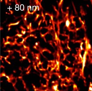
(figures from Arizono et al 2020)





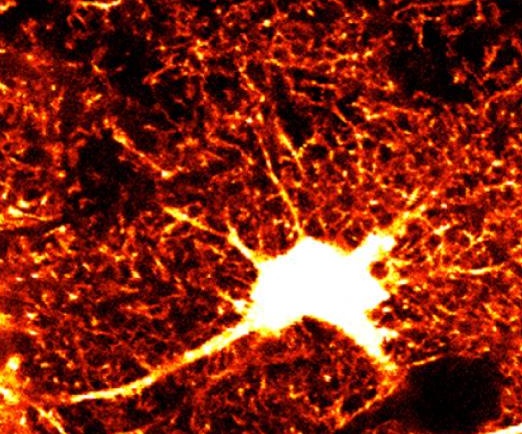
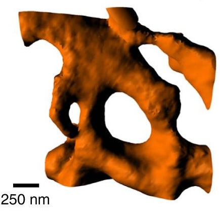
An astrocytic calcium event can be localized or extensive. When such an event happens, calcium is released from the astrocytic ER, causing exocytosis of gliotransmitters including glutamate, across a large number of synapses. What happens next is synapse-specific, there is a diversity of effects of astrocytic calcium on LTD, LTP, STDP, and various gliotransmitters. These are complicated events. They're nowhere near as simple as a Hodgkin-Huxley action potential. Astrocytic activity occurs in a sea of network modes, biochemical modes, and electrical events both near and distant. Machine learning considers the algebraic component in terms of matrices of synaptic weights, and it's already clear that to do anything interesting with them requires their expansion in the time domain (like with transformers). The theory of information geometry links the machine learning algebra with the larger context of moving manifolds, which is exactly what we have in the endoplasmic reticulum in astrocyte leaflets. This provides another layer of geometry, outside of the "connectome" in the machine learning sense. If we're laying down a graph structure on top of a connectionist algebra, an extra layer of geometry allows us to do some amazing things, like pass surfaces through themselves and connect vertices in ways that could never be accomplished with ordinary three dimensional connectivity. The connectivity in the information space is being synthesized by connectivity in physical space.

The other immediate area for fruitful research with astrocytes is their regional behavior, and their regional influence on neural networks. It's often stated in the literature that a single astrocyte can connect with a hundred thousand to a million synapses, and it's also stated that astrocytes tile the brain into non-overlapping territories. These statements are misleading, as there are approximately as many astrocytes in the brain as there are neurons. The hippocampus is a fruitful area for modeling because it has been extensively studied and its geometry and its connectome are well known. An astrocyte is said to contact about 100,000 hippocampal neurons, and this size is about the same as the size of a sharp wave ripple, a characteristic electrophysiological event that is important for both computation and behavior. These are essentially brief bursts of high frequency oscillation, so a region of the network is undergoing a "phase transition" into a different dynamic mode, and this new mode conveys information, it has been shown to be important (for example) in the selection of alternate behaviors in multiple choice scenarios. A calcium event in an astrocyte could be quite sufficient to drive a region of the network into this new mode, affecting the gain through a million synapses at once - and it gets even more interesting when one considers the role of network-wide calcium "waves". Such considerations require the simulator to scale. Scale is the single biggest issue in computational simulations. We're talking about calcium events in 50 nm astrocyte leaflets, affecting the population behavior of neurons in a brain structure that's several cm long. These considerations impose some constraints on our simulations. We'll regularly get numbers in the 1e-13 and 1e-14 range, so it'll help us if we use units that end up closer to 1. An example was already given in relation to standardization around 1 micron lengths, and the principle is the same in all cases, we try to pick a midpoint that gives us a useful floating point range. Even if we use microns, the distance between nm vertices becomes 1e-3^2, which is a small number, and when we multiply this by another small number we sometimes get a condition called "underflow". Different computers and operating systems handle this differently, it's not exactly like division by zero, it doesn't always result in a processor trap. Some systems ignore it and return zero, which is not helpful for us. So these simulations create some issues we have to pay attention to.

Physical theory is simple enough, we basically have three physical laws we're going to enforce on our meshes:

• What goes in, must come out
• What goes around, comes around
• There is conservation of energy, mass, momentum, and charge

The first statement is called the Divergence Theorem and the second statement is called Green's Theorem. The third statement is familiar to all physics students, and in our case it translates into Stokes' Law. On a mesh, complex physics boils down to simple geometry. We're looking at distances between vertices, orientations of line segments, and summations around sets of edges. The computational efficiency depends on the way we can represent the data structures in memory. In the C language (in any of its flavors), we can directly use linked lists, they're fast but they're tricky to program and debug. In Python, we can use lists[], they're convenient to access but they're slow and unsuitable for large data structures. A hybrid concept works well in many cases, for instance a vertex only has a small number of neighbors. The simulator is going to need rapid access to neighbors, and an array will be faster than a list and easier to pass to a GPU, but we'll need to pre-arrange the elements so they're oriented correctly. Some knowledge of these kinds of implementation details is helpful when building models. Eventually, one finds that rotten meshes result in rotten (and expensive) models. One discovers that it pays to pay attention to the mesh up front. Annie's method uses the 1-nm "reference mesh" to generate any resolution required for computation. The initial reference mesh is enormous, it will typically contain 100 million vertices per neuron, and this mesh never needs to be displayed, it only needs to be stored. In the past, if you were working at the biophysical level you only needed a few hundred vertices in a local area, whereas if you were working at the connectome level you'd never need 1 nm resolution. Times have changed. The astrocyte puff changes the network behavior, the butterfly flapping its wings causes the monsoon. The modern concept of simulation requires seamless scaling over 7 to 8 orders of magnitude, one could reasonably say from nm to cm which is 8 orders. You'll make a change at the biophysical level in an astrocyte leaf at a 50 nm scale, and observe its behavior on sharp wave ripples in the hippocampus that encompass multiple mm. Conversely, you'll wish to know how the algebraic behavior of synapses in a neural network affects the geometric behavior of calcium events in astrocytes. If your astrocyte is sitting in the middle of a cortical layer, it'll behave differently than if it's sitting between layers and wrapping synapses in multiple layers.

Annie is a bridge from the science to the engineering. As of this writing (in early June 2026) there is only one other tool that comes close to what Annie does, it's from the Open Brain Institute. It's a wonderful on-line portal that lets you quickly generate simulations and view the results. It has an excellent meshing system but it's expensive, you do it online in the cloud and you get a perfect mesh but it ends up costing you 5 dollars, so if you're doing 100 meshes that's 500 bucks. The easier way is to use Annie to create the mesh you need on your PC, then upload it along with the simulation results. Online you can only use Neuron, which is a great simulator but it's not a finite element engine. Using Neuron your best bet is to use tiny compartments, in which case your simulation once again gets expensive. The easier way is to let Annie run over the weekend on your PC. Relax, have a cup of coffee, go have a barbecue with the neighbors, when you get back your results will be ready and you'll get them for free. If you're mass-producing simulations you're on the bleeding edge of the simulation world, and you're probably in the cloud just by virtue of the sheer number of resources you're using, and in that case maybe you'll prefer the web access and online residency. OBI has an enormous number of raw neuron and astrocyte pictures, as does BOSS and MICrONS, and Annie can't compete (and doesn't want to, she's not in the database business). Getting a mesh from the online form to any portable format is still difficult, so in many cases you'll want to start with an online picture or tracing, and download it and work with it locally. Annie will generate Neuron code to the extent possible, usually it's easy from networks and single neurons but nearly impossible in the biophysical case (because of the underlying assumptions that are hard-coded). You can also try other engines, you can translate your simulation to OpenFoam or any other solver, including the commercial ones like Ansys, but these are multi-physics instead of neuroscience so expect some issues with vocabulary. In practice the initial phase of a simulation is the hardest because one must find the boundary conditions that work, and one must find the range of physical constants that works. The usual starting point is to ascertain the equilibrium conditions in a linear or nearly linear context. This exercise forces us to meet the minimal computational requirements, like properly oriented normals. And, it provides a sanity check for the range of calculation - for example if our viscosity is wildly different from the diffusion coefficients for hydrated calcium ions we have to provide an explanation (perhaps in terms of charge groups attached to larger molecules like IP3 clusters). Charge matters, it creates forces that interact with reaction and diffusion. Charge can slow down or speed up diffusion, and it can create pockets and layers of reaction. In a real brain the Reynolds numbers are low and CSF is almost as thin as water, so we usually model the extracellular space as a sea of ions. The conditions inside the cell are quite different though, in addition to the well known electrical differences and concentrations of cations, there are large numbers of negatively charged macromolecules trapped inside the cell, the positions of which affect diffusion and transport. Viscosity is typically much higher inside the cell.