(this page is under development)

Atrocytes are very smart. They don't "exactly" compute, per se. However they influence the computations of everything around them. It's fascinating and educational to see how an astrocyte wraps an axon. First of all, axons don't simply "exist", they grow from the cell body to find their targets. Sometimes they travel over long distances, seeking the goal and avoiding obstacles. Astrocytes are often in communication with the sprouting axons during this process. Once the synapses have stabilized, the astrocytes enwrap them and lock them into place. But that's not the whole story. Dendritic spines are filopodia, they're highly motile, and so are sprouting axons. These are sprouting axons, in a developing brain. You can see the tiny little filopodia extending like fingers from the growing axon, and the bulbous structures they grow from are called "lamellopodia". Filopodia are very small, maybe 50 to 100 nm in diameter. They have a typical lifespan of about 4 hours, if they don't find what they're looking for within that time they retract again. There are constantly new outgrowths and retractions until the axons find their targets.



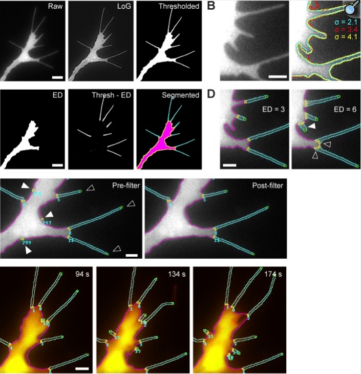
(Figure from Urbancic et al 2017)


Astrocytes are much the same way. Their leaflets are essentially filopodia, they grow until they find what they're looking for, then they wrap. The leaflets have actin skeletons to help maintain their shape. These leaflets are microscope pictures, and look what they're trying to do here. They're trying to generate three dimensional branching patterns. With diameter. Essentially, meshes. The same thing the dendritic spines do. The exact same thing we did with Annie's axons, only... Annie's a lot better at it. She generates a submicron-level mesh in SECONDS. It took less than a minute, end to end, to generate the Blender neuron you saw on the previous page, and it actually works, computationally. This paper here is more along the lines of what we have in mind. Computational modeling of dynamics on a mesh. There are some cool videos on YouTube that show you the real thing.

What exactly is the biochemical environment of astrocytes? There are common elements all over the brain, from the Bergmann glia in the cerebellum to Muller cells in the retina to astrocytes in the hippocampus and cerebral cortex. In general astrocytes have a high potassium conductance mediated mostly by inwardly rectifying potassium channels of the Kr4.1 type. However they're not exactly potassium electrodes, even though gap junctions allow ions to move relatively freely from one astrocyte to another. Firstly, calcium regulates the potassium behavior of astrocytes, and secondly, when it comes to astrocytes, intracellular events are just as important as extracellular events, calcium is sequestered internally and released in bursts into the cytoplasm. Astrocyte membrane resistance is generally low, and membrane capacitance varies depending on position along the tree, the small leaflets with large surface to volume ratios have higher capacitance than the cell bodies. What does the biophysical environment of an astrocyte actually look like?

We can begin answering this question by constructing a model. Our model will use the meshes we've already talked about. We'll model the astrocyte as a bunch of small compartments. Internally these compartments will be parallelepipeds, and on the surface of the astrocyte they'll look like triangles. We are using a discrete geometric approximation, so our volumes will remain on the inside of the surface, and we'll have a tiny discretization error that we can quantify as we decrease the mesh size asymptotically. In this finite element approach, we'll look at the forces on individual molecules, including hydrodynamics like shear and viscosity, inescapable physical forces like gravity, and charge. The hydrodynamic component will involve solving the Navier-Stokes equations in a microfluidic environment, which we can then translate into a Boltzmann model on a lattice (the two views are complementary, and we can verify the seamless nature of the transition by varying mesh sizes). We'll look at results on three levels: the molecular level and the behavior of leaflets, the biochemical level and the effect of astrocytes on synapses (and vice versa), and the effect of astrocytes on the neural network (and vice versa). Our effort will be multi-disciplinary and multi-physical, and we'll compare our results with the literature. Before beginning, let's survey the state of the art, to find out what other people have done so we don't accidentally reinvent the wheel.

The State Of The Art

First of all, there's a nice set of biophysical models pertaining to nerve growth, as shown in the picture above. These models are very geometric, they relate actin cross-linking to the shape of a dendritic spine. (Spines are versions of filopodia, just like growing axons). Spines can change shape in a matter of minutes after intense stimulation, and the biochemical pathway involves several different kinds of second messengers. When calcium enters a spine, it temporarily diminishes motility by inhibiting actin cross-linking. This results in a change in the mechanical forces along the membrane surface (since the cytoskeleton is directly underneath the membrane). Because of this, the membrane flattens out, and the spine becomes more mushroom-shaped, and sometimes it even acquires a small divit. The results of these simulations demonstrate very clearly that mechanical forces are important in the moment-to-moment life of synapses.

To bring charge into the equation, we're interested in ions and trans-membrane ion flows. The paper from Terry Sejnowski's group is helpful because it's the first that attempts to combine charge and fluid flow.


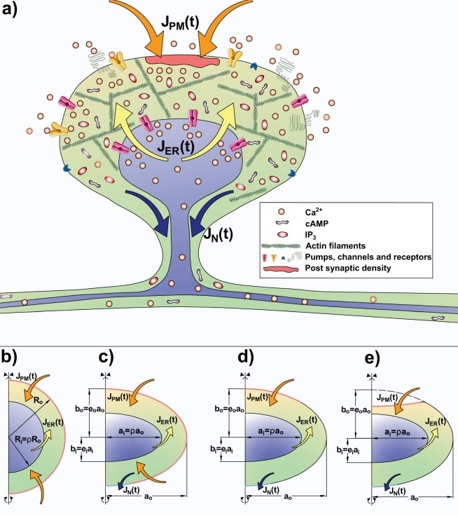
(figure from Cugno et al 2019)

There is a charge-based model called EMI that started by targeting gap junctions in the cardiac syncytium, and rapidly evolved in the direction of the brain. This model is important insofar as it's the first to deal with membrane properties ("materials") in a realistic way. However it makes some outrageous assumptions, like isotropy and homogeneity, that don't apply in tightly packed areas like the cerebral cortex on the home page, or the 20 nm space between neurons and astrocytes. Nevertheless, papers like this come pretty close to what we're trying to do (you'll notice the mesh in their Fig 1).

There are a few models that attempt to deal with membrane behavior at the level of molecular dynamics, however they haven't told us a lot so far. The technology around this is difficult, there is still a big difference between molecules floating around in a sea of lipids, and ion channels opening and closing. Nevertheless these models have had some successes in terms of the kinetics of receptor behavior, especially as it pertains to trauma and disease. Neuroscientists generally agree that there are rapid biophysical changes in neurons and astrocytes during normal activity.

So how does Annie's contribution differ from the existing models? There are multiple obvious reasons why computational modeling of neurons and astrocytes is headed towards finite elements. First, traditional simulation has shown us beyond any shadow of a doubt that connectomics is not enough. The limitations of modern AI are proof enough of this assertion. From a systems standpoint, it is painfully obvious that synapses do not simplify modify themselves in response to input, even first-year engineering students will recognize the intricacies involved in the management of a short term memory buffer. Anyone who's ever studied CPU architecture understands what a cache is, and why there are multiple levels of caching. The brain is no different, the information leaving the hippocampus is different from the information entering it. Secondly, our brains receive overwhelming amounts of information, there are petabytes of raw data entering every day, and only a tiny fraction of that ever gets stored. The filtering and management of what gets stored is still poorly understood. Clearly it has something to with neurons, and it also has something to do with astrocytes, because learning doesn't happen correctly (sometimes "at all") when the astrocytes are disabled. Finite element modeling lets us look at things that traditional simulators have a hard time with, like neuron geometry that requires hundreds of computational compartments, and the poorly understood relationship between circadian rhythms and membrane capacitance.

Annie's primary goal is utility. Finite element modeling of neurons and astrocytes is hard, and it doesn't have to be that way. In addition to the learning curve involved in the math, the nature of the software ecosystem is such that scientists need to become programmers, and even so there's a dearth of working software. There are generally three steps in modeling: pre-processing, computation, and visualization. There are plenty of simulators that can handle the computational part, most of them come from physics, but physics is physics, the same laws of physics apply in the brain as in weather and galaxies. The hardest part is getting your neuron into the simulator, and we've covered some significant parts of that workflow on these pages. First you convert your morphology into a mesh, then you massage the mesh so it's geometrically and topologically robust, then you populate it with materials, and carve out little pieces of it so you can put organelles and molecular structures inside it. Without Annie, you have essentially two choices: you can place your faith in the AI, or you can fight an uphill battle against the open source software (most likely it'll be both). With Annie, you import a tracing and push a button, then wait a few minutes till a perfect computational mesh pops out, which you can then drag into the finite element tool of your choice and permute in whatever way is required for the simulator. Annie will take you as far as the simulation, she's not a molecular dynamics engine. With Annie you can put your astrocytes inside a neural network and make sure they work, before spending all the effort meshing and materializing. Annie cuts through about 50% of the initial workflow, typically she saves about 3 days' work with every new neuron or astrocyte. One of the big problems with finite element modeling is you sometimes don't find out things won't work till the very end, but Annie will tell you instantly if your mesh isn't going to make it. That alone is worth the purchase price! (Which is free!)

Biophysical Model Of An Astrocyte

Let's build a model. We'll go all the way through the workflow, from start to finish. We start with some assumptions. First, our extracellular liquid environment is "nearly" water, it has a low Reynolds number. There have been extensive studies in the vascular literature on the elasticity of blood, it has a small elasticity due to its ionic content and the presence of large proteins and compressible cells. In our biophysical model we will begin with the assumption that CSF is "mostly" incompressible. First of all this assumption greatly simplifies our calculations, it allows us to start in a simple place and we can build up later if we need the complexity. But generally it may be a pretty good assumption, and we'll find out how good it is when we compare our results with real biology. We'll make our extracellular fluid conform to the generally accepted ionic concentrations, which are mostly in the mM range. We can begin with synthetic (or traced) astrocyte morphologies, we'll start with the leaflets which have a large surface to volume ratio and are wrapped around synapses (so they're mostly oddly shaped). The first thing we'll need is an appropriate mesh, so we immediately have to consider the boundary conditions. On the synaptic side the membrane completely encloses the leaflet, but on the cytosolic side we have to make some assumptions about the ion movements (otherwise we have no choice but to model the whole astrocyte, and we want to do something better - we want to use small compartments instead of treating the astrocyte like a point). If we simply chop off the astrocytic branch on the somatic side of the leaflet, we end up with an "open" situation, in which we have to treat what's on the other side as a "reservoir" into which ions can enter and exit freely. Our other choice is to seal off the wound by putting a piece of plasma membrane across the cut. In this case the inner boundary becomes "closed", and we treat the downstream ionic interactions the same way we treat the leaflet. At a scale of 50 nm, it's not entirely clear which way is more realistic. Probably there are aspects of both, the pathway to the astrocyte soma isn't entirely closed but it's cluttered, there is geometry and there are plenty of large molecules. We can begin by treating the somatic side of the astrocyte as one large compartment, homogeneous but separate from the extracellular space. This means our plasma membrane becomes essentially a half-shell, closed on one side and open on the other. This is a very common situation in finite element modeling, there are plenty of existing examples to draw from.

We are in three dimensions, and we'll call our volume Ω according to convention. Therefore our plasma membrane will be the boundary, it will be dΩ. Our three fundamental physical principles are, that the volume is constant (principle one), that interactions are local (principle two), and that forces add (principle three). The fundamental piece of math we'll use is Stokes' Law, which states that what happens in the volume is reflected at the surface. This lets us convert integrals over the volume Ω to integrals over the surface dΩ. We have the convenient relationship ∫_Ω dF = ∫_dΩ F, and on our mesh a derivative is simply b-a and an integral is just Σ (b-a). We will have some non-linear terms, that we'll attempt to remove and convert to a nice linear system of the form k U = F that we can pass to a linear solver.




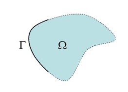
We being by outlining our physical constraints. Let us consider one volume, our volume Ω. Our first physical law (the Divergence Theorem) states that anything leaving the volume must enter other volumes. Engineers think of this concept in terms of "sink" and "source". If there is a source inside the volume, there must be a sink somewhere else. In our model, the ultimate sink is the extracellular space on the open side of the astrocyte branch. The forces in our model are pretty easy to understand, we have mass, charge, and the hydrodynamic forces like viscosity. If we make the assumption of incompressibility we can already get rid of a nasty non-linear term in the Navier-Stokes formulation. And while we're doing this, we don't want to do anything that will preclude us from moving over to a Boltzmann lattice at the drop of a hat. Therefore we'll be more explicit than simply talking about the "concentration" of an ion. Instead we will talk about how many ions exist within a given volume of mesh. If one ion enters, one must leave - resulting in a very simple formulation in our code: if nIn == nOut then our divergence constraint has been met, otherwise we have a source or sink somewhere. You can already see what's going on here, we're setting up our math to be as simple as possible so the simulator can blaze through it. In fact as we'll see, the most complicated thing we have to calculate is the cotangents of mesh elements, and we only have to do that once. The rest of the time, we're just adding and multiplying numbers (and maybe dividing by two, or three, or six). This makes the computer's life a lot easier, and it also lets us take advantage of parallelism by splitting the workload among many computers, since all the calculations are local.

Next we will set up the boundary conditions along our plasma membrane. This is where the ion channels live, so we will have some selective charge and mass transfer across the membrane. We'll bow to Mother Nature and treat all channel activity as stochastic. There will always be a "probability" of opening or closing, there will never be definiteness about it. Stipulating the probability is never exactly 0 or 1 gives us some interesting mathematical capabilities, for instance it lets us reshape probability distributions and scale their ranges. This is what an ion distribution might look like when a channel opens. It looks a lot like the intracellular distribution of glutamate after uptake by EAAT's. The diffusion is described by the Navier-Stokes equation with low Reynolds number and near-zero vorticity.



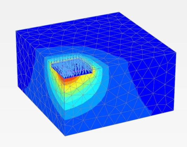
In the figure there is a small patch of membrane populated with channels, and the local ion concentrations are shown in color. If you look closely you can see the field normals associated with each channel. The patch of membrane was created with the material-based mechanism discussed earlier, the unified tetrahedralized mesh was partitioned to accommodate the patch, and the patch was then endowed with additional physical properties (channels). The translation of vocabulary between neuroscience and physics is often the biggest challenge. Neuroscientists think in terms of stimulation, physicists think in terms of forces. When you're looking at the screen, the text says "forces", not stimulation level. In our simulation, we'll have two sets of membranes right next to each other, separated by a tiny space only 20 nm wide. So the normals you see in the above diagram, will be pointing straight at another membrane. In real life "straight" is a give or take, for example the EAAT clusters in astrocytes aren't "always" perfectly normal to the synapse, but they're always very close by and in all cases they live in the tiny pericellular space surrounding the neuron. Physically though, it's pretty clear that a cluster at a 45 degree angle will respond differently than a cluster that's perfectly orthogonal.

Before starting, we should say a word about differentiability, because it's a big deal, especially in machine learning. The artificial networks in use today (with a few neuromorphic exceptions) depend on the back propagation of derivatives related to energy functions, and it was pointed out long ago that this is non-biological because synapses don't talk backwards. Well... it turns out that in some cases they do, and there are other ways of talking backwards besides just synaptic... however let's set that aside and consider that in the primary mode of feed-forward synaptic transmission the backwards propagation of derivatives is problematic. On a mesh though, the computation of derivatives becomes easy, in fact it becomes explicit, because it's a byproduct of the calculations. We would like to engage in the business of derivatives because subtracting the value of a function at two points is the same as integrating the derivative over a path between those two points. This is how we get the velocities of particles (ions) in a fluid, and if we're really serious about the stochastic side of things we have to do this using Brownian motion (adjusted for the physics), which involves the generation of an enormous amount of random numbers at each time step. Tracing the path of molecules is like ray tracing in computer graphics, the results are spectacular but it takes a while. And this, takes us right to the heart of the simulation business - which is: what kinds of tradeoffs do I need to make, to get my simulation to run correctly, so I get results sometime within my lifetime? We're talking about molecules that are 0.1 nm big, floating around in a sea of liquid and charge and other stuff, and we're going to look at that on a mesh that's about 1 nm big, so we may have 100 or more small molecules floating around in that volume - which is not "really" enough to do statistics on - so we should really either increase our mesh size so we can do statistics, or decrease it so we get fewer molecules per volume. We can't really do the latter, it would be heading in the wrong direction - we want faster simulations, not slower, and at this early stage we have no reason to believe we'll gain anything from the increased computation. So let's go the other way, we'll make our mesh... say... 10 nm. That'll give us at least a thousand small molecules to do statistics on, and it's also small enough to give us 10 volumes over the span of a PSD. It seems like a good price point between sufficient precision and computational overkill.

Now, to the boundary conditions. How do we model our plasma membranes? We have three of them - we have an astrocyte, and a pre- and post-synaptic neuron. In our simulation, we're going to do three things in order: first determine the equilibrium conditions, second determine the dynamic response by perturbing the equilibrium in various ways, and third program the astrocyte to generate a calcium puff and observe the effect is has on the synapse. (And that's just the beginning, we can move on from there). The primary feature of plasma membranes is their membrane-bound molecules, which includes ion channels. We can greatly simplify our calculations by assuming that all flow through channels is normal to the membrane surface. (We have the unit normals already, we had to calculate them when we created the mesh, to properly orient the faces). The assumption underlying the assumption, is that if a channel is not perpendicular then it's not yet working, it's either being inserted or it's dysfunctional. Those are probably reasonable assumptions. The question then becomes how we're going to model the extracellular space between the membranes. From a microfluidic perspective this space is so small that an ion emitted transversely will not diffuse very far. There is force associated with ion transfer, an ion emitted from a channel will have some momentum in the forward direction, which will primarily determine its diffusive behavior unless the nearby fluid flow has a high velocity. Microfluidics considers "droplets", which in our case are very much like hydrated ions. They can be modeled as computational units because they're distinct from the surrounding water, they have mass and charge. Similarly at the synapse, we want to look at the diffusion of glutamate out of the synapse, and in this case we're looking at the near-simultaneous expulsion of thousands of charged glutamate molecules into a narrow scaffolding - so many that a substantial fraction escapes and diffuses out of the cleft. It then either spills down the shaft of the spine in the extracellular space, or gets sucked out of the extracellular space by the astrocytes via their EAAT's.

It is noteworthy that some of the previous simulation efforts have ignored the charge component. Calcium is charged, and so is glutamate. When an action potential arrives at a synapse, there is a rapid current shift in the synaptic cleft. First calcium flows in, then glutamate flows out, so the charge in the cleft goes one way and then the other. We already noted a "memory" effect in the AMPA receptors, in the form of adaptive gain control. This is an interesting computational device, it makes the transfer function sigmoidal (logistic, or at least biphasic), and it would be interesting to know whether it's being kept in the linear range or whether there are times when it moves to the extremes. While this is going on, the astrocyte is buffering the potassium that got expelled from the synapse during transmission. This is a whole complicated story by itself, because there are different channel types on the neuron side and the astrocyte side, and each side has multiple types, and the particular composition varies by brain region. We'd like to start simple, by accounting for the major currents. Unfortunately, there are a dozen receptor types in the presynaptic membrane, and they all co-exist and they're all active during synaptic transmission. The T, L, and N/P/Q/R types of calcium channels all have different voltage sensitivities with different kinetics. A traditional simulation like a NEURON patch gets to abstract all these away with channel densities, but we don't get to do that. On a mesh, channel densities are reflected by vertex and face behavior. Channels are computational entities, depending on the density some mesh elements may have them, some may not, and some may have more than one if we allow it. Sometimes we run into computational difficulties if we put too much on a node, there are non-collision algorithms that ensure our channels are appropriately spaced and don't interfere with each other. So what we have to do is run an algorithm that attaches channels to nodes, and checks for conflicts and adjusts accordingly. In a way this is very close to what we do when we sample a mesh. In this case we'll sample a vertex, attach a channel to it, and if there's already one there we'll move it over, and if we run out of room we'll raise a red flag and tell the user to reconsider.

Great, so now we have a bunch of channels on a mesh. Now what? Well... now we have fluid flow, and charge, and synaptic inputs. We can do the diffusion first, that's a good starting place. The more general context for diffusion is "reaction"-diffusion, which frequently includes non-linear terms that complicate our simulation and we'd like to get rid of. An example is the part of Navier-Stokes that relates to vorticity. In the brain, we're probably not going to have any vorticity. There may be some minuscule edge effects but generally the velocities and pressures and Reynolds numbers will be too low for vorticity. To simplify the diffusion portion of our calculations, we can simply ignore the vorticity, that's a brute-force approach but it might be okay to begin with. If we add charge to the remaining equation, we get a version of the Poisson-Nernst-Planck formulation, which is well known in electro-hydrodynamics. The good news here is, we can take this formulation to just about any simulator, including OpenFoam and Moose. One can find dozens of existing EHD simulations online, and plenty of examples to draw from. But this is where it gets tricky, because now we have to consider the actual physical geometry. We have to reconcile the direction of ion movement with the structure of our mesh, for instance we have transverse ion flow across membranes but our mesh is triangular, so we end up having to calculate dot products and inner products on every element. This is where the nasty issue of isotropy rears its ugly little head. And we really have to think about this in detail, because it's going to make a big difference in the complexity of our simulation, and ultimately it's going to determine whether we can hope for results this year or whether we have to pass the whole thing on to the next generation.

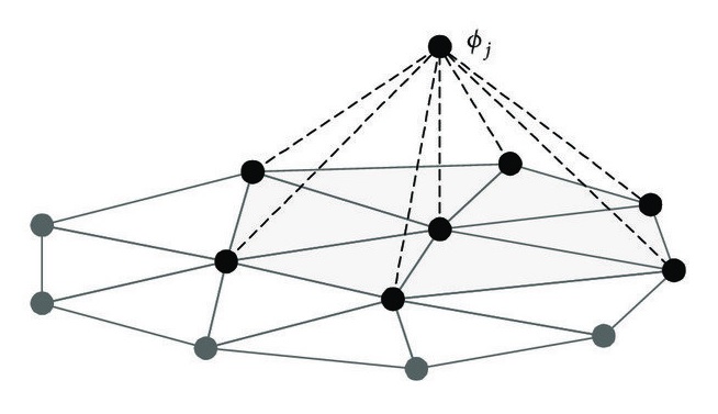
Historically, the assumption of isotropy is what's gotten us this far. It's what allows gigantic simulations to run "at all", even on supercomputers, and it's what allows little ones to run on NEURON. One can think at a mesoscopic level about the uniformity of ion concentrations, so for example if we're modeling our extracellular space as an ocean of unlimited seawater we always get isotropy (a uniform pattern of concentration in any direction). However if we have a tight mesh and the neuron next door is only 50 nm away, it's very doubtful we're going to have isotropy. At a synapse, we might have isotropy within the 200 nm extent of a synaptic web, but we're not going to have it along the edges, where there are tiny cisterns between the neuron and the astrocyte, and channels are clustered along well defined attachments between the two membranes. This consideration takes us back to mesh size, because if we're making the statistical assumption we require isotropy within our statistical unit, meaning within each volume of our mesh. This constrains us to handling "average" concentrations within the volume, and in fact that's exactly what we're after with the finite element approach. The average within a volume on a mesh is exactly the "d" we were talking about earlier, the tiny little increment that we consider to be linear when we're doing the math. In our mesh volume, everything is linear. So now, let's talk about how we get from a non-linear "function" (some kind of vector field over the mesh, that we're interested in, maybe charge, or maybe ion concentration) to a linear version we can compute. The point of the mesh is, we have a "field" (it could be anything, it could be a scalar like temperature, it could be a vector like fluid velocity, or it could be a tensor like electromagnetic force) on the mesh, and we'd like to know what that field is. The field is a solution to a set of partial differential equations, and the simulation is going to show us how the solution develops in time and space. To approximate the function on our discrete mesh, we have to discretize the function too, and we do that using what's known as a "Whitney basis". The Whitney basis has a value of 1 at the vertex, and 0 at all other vertices. Between the vertices, the value is extrapolated, so between a vertex and its neighbor we have a straight line in both directions. This is a "piece-wise approximation" to a surface, it's going to give us an extrapolated picture of our function.

Apologies in advance, but this is where the pedal hits the metal and we have to get into some hard core math. To keep things as gentle as possible, we'll just look at the landscape. When isotropy no longer applies, the k matrix above (sometimes called a "stiffness matrix") becomes a tensor, it acquires more dimensions and more degrees of freedom. This makes the discrete solution unstable, in particular the computations cause spurious oscillations that arise because of the grid rather than the physics. (This problem is well known to anyone who's ever played with Wilson-Cowan). Essentially what happens is the Dirichlet boundary conditions become Neumann conditions instead, which are "softer". Over the years many methods have arisen that further constrain the computations so they can be solved, for example the inner product can be extended to the L2-integrable space and the basis functions changed to accommodate least squares, the k tensor can be restricted to be symmetric which lets us look at flows in porous media (like membranes with channels), and there are dozens of modifications of the basic Galerkin method like Streamline Upwind Petrov, but there is some reluctance to use these methods because they're artificial (although the same thing could be said for renormalization in most of physics, it's kind of like the global energy function in a Hopfield network, everyone recognizes the need but no one knows how it's supported). Another stabilization method is mesh adaptation, sometimes if you change the grid you can get rid of spurious oscillations. Yet another method is to introduce enough noise to bury the oscillations. This latter method is interesting because it cross over into the molecular domain, where we can model diffusion in terms of Markov jump processes. Here, the noise is directly affecting the jump probability so we can control the diffusion by controlling the noise. These are methods for numerical stabilization, and we don't want to use them unless we have to. The reality though, is if we don't want to use them, we'll need very tight control over our simulation parameters. We would like to use a method that will work across the board, so when we're changing our mesh size to study discretization errors, the simulation doesn't suddenly go out to lunch and start oscillating wildly.

These are good reasons to start simple. One can usually begin with the linear case, just to get an equilibrium. In our case, we'll say that the force on any particle is the sum of the hydrodynamic force, van der Waals forces, and electromagnetic force. This multi-physical approach lends itself well to both computation on meshes and stochastic representation using a master equation. The simplest way to start is with a lattice (a grid). This reduces the entire problem almost to the level of undergraduate civil engineering. We can have Annie create a grid for us, and the great thing about that is when we're ready we can simply replace the geometry with the mesh. With one button-push we can see whether things still work when we apply our mesh geometry to the equations. If we tell Annie EXTENT=10 we'll get 21 vertices along a dimension (10 in each direction plus 0), that'll give us a little over 8000 nodes on a three dimensional lattice. Each voxel in the grid becomes a computational element, and since everything is in square arrays we can efficiently represent them and access them in the computer memory. At this point, the numerical simulation becomes irrevocably bound to the geometry, so when we want to replace the grid with our real mesh, this is where we start. We now attach data to the vertices, edges, and faces. Each has its own computational requirement, depending on what exactly we're looking at. Ion flow in a liquid is a vector field with directions on the mesh, whereas electrical potential is a scalar field that can be calculated at the barycenter or integrated over the boundary. In general we'll have a data structure consisting of an arbitrary arrangement of numbers, and we have to tell the simulator what to do with those numbers. A simulator doesn't want to see variables like x and y, it's too expensive to push those onto the stack for function calls. The simulator wants to see a pointer to the base of an array, and an equation that says array[0] * (array[2] - array[1]). So we have to convert our physical equations to a language the simulator understands. In a way it's no different than what we did with meshes when we calculated the Hodge star. (Did we do that? I forget. If not, I'll put in another plug for Keenan Crane and his colleague Justin Solomon). With meshes, we had to be careful with the orientations, and it's the same way with the calculations because the most common issue is a sign inversion in an integral somewhere. At this point in the workflow, the computational integrity depends on the integrity of the geometry - which is why we paid so much attention to it, and checked it six ways from Sunday to ensure it was manifold and didn't have any holes or dangling edges. If your mesh isn't manifold and watertight, don't bother trying to do any calculations on it. So now, what to do at the boundaries? Well... we have choices. A lipid bilayer membrane is frequently modeled as three layers in biophysical simulations - two charged layers containing the hydrophilic heads of membrane bound proteins, and an elastic layer in the middle consisting of phospholipid tails that gives the "fluid" mosaic model its name. If we "skin" our lattice with a lipid bilayer, we come back to the question we asked earlier, which is what are we going to do with the somatic side of the leaflet? Apparently, we have to leave one side of the cube open, so on that side we have to use Neumann boundary conditions, whereas on the other side we can use a Dirichlet condition. If we do things this way, our ion channels will end up being inserted into the boundary layer, and it therefore makes sense to use a boundary layer with the same geometry as the inside, so we can easily transfer physical quantities. This setup also provides a natural relationship with the Nernst and GHK equations known to neurophysiologists, they can be pretty much directly applied to patches of membrane.

To get our results, we would like a basis function "per point", so we can simply interpolate and add the results from each mesh element to get our final visualization. The requirement on the basis functions is therefore that they satisfy a Kronecker delta, that is, they're 1 at their vertex and 0 at every other vertex. There are many functions that satisfy this relationship. Keep in mind that we're trying to find a function (the solution of the Laplace equation on our mesh, or whatever the electro-hydrodynamic equations end up looking like), and we're trying to get the shape of that function by breaking it up into little tiny parts and computing each part. So our basis functions need to be continuous over the boundaries between elements, which we get for free with the simple Whitney functions (at least they're piece-wise linear), but things get a little weird when we start considering all the possible L2-integrable functions that might satisfy such a relationship. For example if we're breaking up the electric and fluidic components, we should make sure that our basis functions are compatible with both sets of calculations. In the electromagnetic world there are the Nedelec functions that guarantee the tangential continuity of vector fields across element boundaries but allow the normal components to be discontinuous. Here's a quick look at some sets of basis functions:



Our choice of basis functions is more than theoretical. For instance the ordinary Lagrange functions won't work so well when we move to Neumann boundary conditions, because the numerical solvers become unstable. So we have to use basis functions with friendlier convergence behavior. There are basis functions that take on non-zero values between the vertices, that still satisfy the requirement that they be non-zero at exactly one vertex and zero at every other vertex. The part of the workflow that tests basis functions and determines which one(s) to use is covered very nicely in the deal.ii documentation. One first ascertains that one understands the behavior of the function in a linear context, then one builds a multilinear form representing the left hand side of the equation and maps it to the mesh. Finally when one "turns on" the entire mesh, one hopes not to be surprised by entirely new spurious behavior. Before to moving to more complicated geometry, one may wish to begin assessing the discretization errors by adjusting the mesh size and spacing and plotting the resultd to see if there is an obvious asymptote. Usually the target mesh is more precise than the test mesh, so we may also wish to increase the mesh density before changing the shape. The first result is always exciting. "Look ma, it works!" But that's when the real work starts. Once you've ascertained you have a working simulation, you can begin with the science. Without doubt, one of the first things you'll encounter is conditions under which the simulation will break. The easy way to break a simulation is to make the time constants very small, so the number-cruncher has to divide by near-zero all the time. So there's an initial phase where you play with the units to get them in a nice comfortable range. Unlike some simulators, Annie's not going to be responsible for your choice of units. You're going to have to find numbers that work anyway, and at the end of the day you'll have to research your units to make that happen, and the best thing you can do is find numbers that give you a nice solid baseline from which you have a working range in either direction. When something stops working, you're going to have to determine whether it's because of the physics, or because of a broken simulation. So you treat your simulation just like a live experiment, you implement controls, and you rule out the other possibilities. In the infamous words of Arthur Conan Doyle, "when all other possibilities have been eliminated, whatever remains, no matter how improbable, must be the truth". Like Mr. Holmes, we have no advance ground truth to draw upon. However we do have 150 years worth of observations, for comparison with a similar system and to discover the differences. Brain research is one of the last frontiers of science. Right now, we can't even answer the most basic of questions, we're still in the stone age, we haven't even invented the vacuum tube yet. Why is red "red"? No one knows. We haven't an inkling, not even the foggiest clue. However we can see parts of the brain light up when we pay attention to things, that's a start. :)