In a mesh setting we're dealing with partial differential equations that describe relationships in space and time, and occasionally we have some additional complexity with ordinary differential equations around the boundaries. Biophysical equations specifically include interactions of the reaction-diffusion variety. This topic merits some discussion, because these terms have carried various meanings over the years. Lately there's been an explosion of neural network models based on dynamic attractors. That word "dynamic" has many meanings. Neurons in networks acquire additional degrees of freedom, they can do things "relative to the population" that they can't do on their own. Phase encoding is an excellent example, and phase encoding implies the existence of a periodic signal somewhere (an "oscillator"). Neural oscillators are subject to entrainment just like pendulums on a bar, and this behavior is described by the Kuramoto model of phase coupling. The difficulty with the Kuramoto model is it's only single-frequency, and it's been solved for some special biphasic cases but in neuroscience the phase-related behavior of subthreshold membrane oscillations is well known. It occurs at all frequencies, especially those in a range around the equilibrium that tend to entrain towards the mean. We have a bunch of little oscillators at every point in space, and the exact timing of an action potential is going to depend on those oscillators in complex ways. Every functionally coupled pair of voltage-dependent ion channels can form an oscillator. Many of the computational simulations performed to date indicate that the precise spike timing of a neuron can be influenced by electrical coupling from neighboring neurons. And if we're seeing this in axons we'll see it in dendrites too, we'll get similar behavior in every dendrite that generates mini-spikes (which is probably every pyramidal cell in the cerebral cortex and then some). If, say, we were looking for a way that a neuron might be able to memorize and reproduce a spike train, this would be an excellent place to start looking.
There is some further discussion around this point. Lately there's been a lot of talk about "energy functions", what are variously called cost functions, or error functions, or Hamiltonians or Lagrangians, depending on your discipline. In a nonlinear thermodynamic mesh, the covariances described by coupling functions provide another source of non-local interaction, which in this case is more often deemed to be "regional" rather than "global". In relation to things like dynamic neural attractors, we're interested in what determines the size of the attractor, and its shape. Certainly the network geometry does, but in nonlinear meshes one sees standing waves that result from coupling, and in some cases this behavior can be computationally useful. One can do math on a mesh full of oscillators just like it can be done in a Hopfield network, but now there are additional degrees of freedom because of the phase relationships. The point being, that the idea of a "global" variable is still non-biological, there is no such thing known to exist in real brains. What does exist, are "regional" variables, like ion concentrations in the extracellular space, and significantly, the activity in a regionally connected population of astrocytes. It is very likely that dynamic regional boundaries are computationally significant. Some of this is already visible at the level of dynamic attractors, but there's more to it. We need to able to visualize the actual computational boundaries in the simulator. And that is a very tall order unless everything is on a mesh. Simulators of the Brian2 variety aren't going to show it to you. TensorFlow doesn't come close to any such thing. The computational need is to relate the observed behavior to the information geometry. We're looking at the same thing the biologists look at when they poke electrodes into a live brain - we're looking at spike trains. With the simulator we can see a little more, we can see the local extracellular space too. But on a mesh, we have the keys to the kingdom. We can see everything. We can see exactly how those spikes got created, and where they came from. We can actually visualize a volley of spikes in relation to a traveling theta wave. Without a mesh, that's just about impossible. With a mesh, we get it for free.
Membranes
Finite element analysis on nerve membranes is not a new idea. The compartmental models of Wilfrid Rall (late 50's and early 60's) are an early form of the mesh concept. Meshes are simply very small compartments, and there are things we can do with meshes that we can't do any other way. Meshes are reappearing in a big way in the world of neuroscience, as people realize that neural information is not just activity levels, and in fact the interaction between activity levels and the intra- and extra-cellular environments are what distinguishes neuroscience from machine learning. Finite element methods have had some significant successes to date, for example a recent paper describes how extracellular stimulation actually works on a neuron (Fellner et al 2022). Similarly, there is medical interest in the details of stimulation effects on peripheral nerves (Pelot et al 2018). The Pelot group at Duke University is a good read, they're doing a lot of work with these models, and you can find some of their software on GitHub. Finite element models are also one of the few ways to link mechanics and electrical activity (Vasas et al 2024). The concept of "simulating a nerve network" has already outpaced the current state of machine learning in many ways. Neuroscientists as a group are keenly aware there's a lot more to neural networks than just matrix multiplication. And people are starting to figure out how to model syncytia, where you have small synapses embedded into a much larger continuous network (Jaeger and Tveito 2026). Meshes and finite element methods are required for these kinds of investigations, as they extend well beyond the traditional view of neurons as point-like electrical generators. In many cases, computational meshes provide surprising insights, for example one recent paper was able to show that the location of the axon initial segment can be predicted on the basis of the Laplace-Beltrami operator, solved over the neuron shape.
There is a fundamental difference between solving equations in model neurons, and solving them on a mesh. They're only the same insofar as the simulator can crank through each point performing calculations. In IAF neurons, there's only one membrane potential, but in compartments or on meshes, there are many, and they all have to be calculated individually. How you approach this is a question of your workflow and your scientific need. Meshes take time. If all you want to do is a little machine learning with some geometry, you don't really need a mesh, you can just tell Annie to build a simple network of the kind we saw on the first page, and start your simulation. Neurons and synapses compute more or less the same way (since their membranes are similar), but when one starts looking around at how the simulators actually handle this, one becomes horrified. Refractory periods are artificial, they don't happen because of the membrane properties, they happen because of a computational rule that says "remain dormant for 1 msec after firing". Synaptic behavior is determined by exponents that represent the cumulative activity of thousands of receptors, ligands, and who-knows-what-else. In a way, this is like artificially staging the timing within your network. And when done this way, it doesn't tell us very much when something succeeds. It's like, "look, it works!" - well yeah, that's because you programmed it that way. When you get 200 Hz oscillations it's because there's a time constant or a synaptic weight somewhere that's forcing the network into the dynamic. Maybe the astrocytes are sucking all the calcium out of your extracellular space, whereas you're off trying to explain the lack of dendritic spiking with synaptic inhibition. Accounting for all the factors that can affect ion concentrations in a neural network is still difficult, and we need the tools to be in place when the science is ready, because biologists (with very few exceptions) are not computer programmers and they don't have a whole lot of time to spend learning about software. It's more like "can this tool do what I need", and what's needed these days is a lot of visualization and some easy-to-access domain-specific analytics.
The benefit of simple neurons is they're easy to calculate. The complexity of your network can be measured as the ratio of computer time to real time. If a computer tick represents 0.1 msec and it takes an hour to complete, you have a complex simulation. A few years ago, IAF neurons were state of the art, and there's not a whole lot to them, typically their equation is something like:
dV = 1/τ * (Vr - Vm)
so when your membrane potential Vm is above the resting potential Vr, you get a negative correction that forces it back down towards the resting potential. The time constant τ determines how fast the correction occurs, with a long time constant the incremental corrections are slow and it takes a while to get back to the resting potential. This is simple enough, and it's also where the problems start. Inputs are currents, they're movements of ions from one side of the nerve membrane to the other. The movements determine the concentrations on each side of the membrane, and that's what results in a trans-membrane electric potential (a "voltage"). A "voltage" represents a ratio of ions. If we add or remove ions on either side of the membrane, we change the voltage. This is a very different concept from directly linking synaptic inputs to dV. In some simulators, inputs are multiplied by synaptic weights and the result is directly applied to what would otherwise be a GHK equation:
dV = 1/τ * (Vr - Vm) + I(s)
where the I stands for synaptic input instead of ionic current - the assumption being that the synaptic input will directly drive the corresponding current. Which is not always a good assumption. If you have magnesium ions blocking your channels your synaptic behavior relative to the generated currents might be a little different than the equation. It's important to be able to match the equation to the behavior. There are always underlying assumptions, and one must be explicitly aware of them rather than trying to sweep them under the carpet. Even the computational method used to solve the differential equations can sometimes affect the outcome of an experiment, so it's important to have access to a large library of methods and to be able to quickly and easily access them. How do I tell Annie to change the computational method? Easy. METHOD EULER. That's it, that's all. You can use that at the level of the simulation, the network, the cell, the neuron, the synapse, the ion channel, and any other computational object you can attach to a mesh. RK4 is a popular method, because it offers a reasonable compromise between accuracy and performance. There are methods that are computationally precise and almost never blow up, but they can also slow down your simulation. So Annie offers you a choice, choose the method that best meets your needs.
Synapses are the same way. They're traditionally modeled as a biphasic (usually bi-exponential) rise and fall, which is reasonable as far as it goes but if you have modulators or other external factors influencing those times you'll need to account for them somehow. A typical synaptic profile might look like this:
S(t) = Smax * A [e -t/τ1 - e -t/τ2]
where t1 and t2 are the rise and fall times. It gets a little more artificial when one has to introduce synaptic delays, which usually end up like
e -(t-τd) / τr
As you can see, this approach involves a lot of assumptions and a lot of compromises. It works, insofar as it generates what look to be superficially realistic results. But they're not really good enough for comfort. They're good enough to look at and say "okay, it's possible", but they don't speak to how the biological system actually works. What we'd like is, a method that's just as efficient but a hundred times more accurate. And, it turns out, this is within our reach. Using the methods of discrete differential geometry, we can reduce complicated multi-dimensional physics to simple traversals around mesh elements. We can also do some things up front that save us plenty of computational time later on. The result is, that in approximately the same time NEURON can calculate ordinary differential equations, ANNIE can solve partials on a mesh. Biophysics unquestionably takes longer than cable equations, that much is true - however the differences can become very small when we take advantage of the opportunities that are available to us with the discrete exterior calculus. Using DEC we can discretize the entire geometry in a linear or nearly linear manner, avoiding the need for complicated higher order finite element basis functions.
Visualizing Results
A refined computational approach to simulation involves biological realism. For example, in addition to traveling down the axon, action potentials travel antidromically ("backwards") up the dendritic tree and into the apical dendrites, where they affect the ongoing behavior of voltage-dependent calcium channels and so on. In the hippocampus this behavior guides the timing of action potentials relative to theta. The 1-msec travel time from soma to dendrite is significant, it changes the network behavior. On a typical pyramidal neuron there are tens of thousands of dendritic spines, some of which may notice the action potential - so the timing of the incoming volley is crucial. One can certainly engineer this, by programming the time constants and delays - and it is legitimate to ask about the range of time constants needed to support some desired behavior. But at some level programming synaptic delays is cheating, they should be self-determined, not programmed. And the only way to do that with any kind of precision, is using a mesh. Otherwise, we are assuming that each synapse is isolated, and each neuron is isolated, and that's almost never the case in real life. Here is an effect that neuroscientists have known about for years but never fully explored - the modulation of spike timing by ephaptic transmission. Astrocytes form their own electrical syncytium, they're also likely to have significant effects on spike timing. Here's a model showing the dramatic effect on spike timing of simply moving the electrode around.
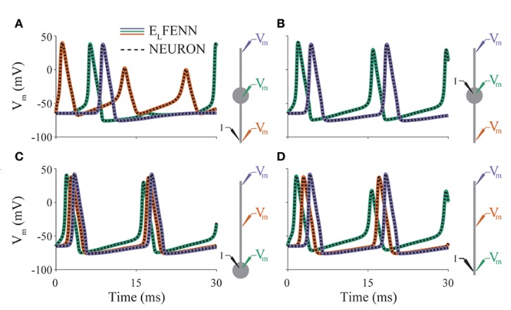
(figure from Shifman & Lewis 2019)
In the interest of realism, when we look at a simulation we need to use all the same tools the physiologists use when they're looking at live brains. FFTs, power spectra, coherence maps, that kind of thing. Visualization. The prerequisites for computability include persistent named objects and the ability to attach arbitrary data to mesh elements. Neurons and astrocytes have their own special issues, which aren't fatal but they can be tricky to deal with. After doing biophysical modeling for a while, one begins to realize it's like playing a musical instrument, you can do everything right and still not get the beautiful results. The end product is a combination of you and the math and the computer... how can I say this... there's a very technical set of papers by the folks at AMES and Sandia, describing some of the many tricks they had to use to get their space shuttle simulations to work. Some of these "tricks" were later proven to be useful mathematically, and now there are libraries full of these things and you can try them in any order.
For instance, this is Lava-DNF, one of many available neural network simulators that provide spiking neurons and connection geometry.
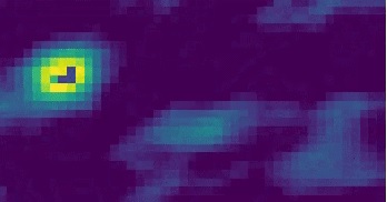
Looks just like Annie, right? Looks exactly like the picture on the Introduction page. They're after the same thing - a heat map of network activity. And, you can see their grid, it's just like Annie's 2-D retina. But that's just it, it's 2-D. Realistic neural networks are three dimensional. The fields are generated by networks that involve all six layers of the cerebral cortex. And neurons in small populations have a lot of issues that have nothing to do with their ion channels, like edge effects due to connectivity (you can clearly see the edge effects above, in biophysical simulations these are called "discretization errors"). Unless these are carefully accounted for, they will affect the behavior of simulations. Large faces are problematic, the grid size needs to be very small, like the meshes on the previous page. Traditional simulations typically resolve the network at the level of the neuron and the synapse, as shown above, however Annie has a much more flexible model in that every grid element is a differential form, it measures a biophysical quantity in a small region of the mesh and it can be positioned, scaled, and rotated as needed.
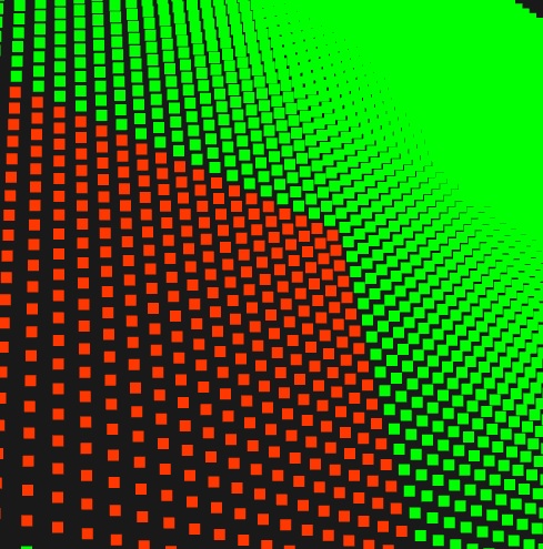
Real brains are three dimensional! Everything in a real brain has volume, there's no such thing as an "infinitely thin sheet". The volume may be small, but it's important - especially when one considers its relationship with extracellular ion concentrations. 3-D visualization is essential for neuroscientific modeling. There's really no point in creating two-dimensional models, even when one believes one can somehow abstract away the unwanted degrees of freedom. So in a way, everything we just showed in two dimensions, is scientifically worthless at this point - and this includes the majority of neural network simulations published between 1985 and 2025. Why? Because they're all two dimensional! Neurons are abstracted away as points, synapses are treated in isolation, and there is hardly ever any consideration of volume conduction, even after the literature shows a noticeable ephaptic effect (even in a small bundle of topographically aligned axons). Those of you with a geometry background may have noticed another interesting aspect of Annie's visualization: those little squares in the picture on the right, are actually differential two-forms, you can see their orientations relative to the grid.
Finite Elements and Discrete Exterior Calculus
Using the exterior calculus, we're going to do things a bit differently than most finite element simulations. A lot of it has to do with the geometry of our mesh elements. We're going to use a topology where vertices are affinely independent, meaning we'll use triangles for surfaces and tetrahedra for volumes. This may seem odd at first, to those who are used to cubes and hexahedra. However the affine construction offers many computational advantages, including the ability to use simple Whitney bases where otherwise some complex higher order polynomials might be needed. Physically we're solving partial differential equations, and on an affine mesh these equations are often reduced to simple addition and subtraction. A differential is just the the value at B minus the value at A, and an integral is just a circulation around the edges surrounding a vertex. We build differential forms from simple elements, edges from points, faces from edges, volumes from faces. Each of these relationships has an incidence matrix we can conveniently represent in signed form with a -1 any time an edge leaves a vertex (for example), and a +1 any time an edge enters a vertex. A weighted sum over a set of vertices (an integral) thus reduces to a simple matrix multiplication.
Finite element and volume analysis can look a little daunting at first. Compare these equations to those for an IAF neuron:
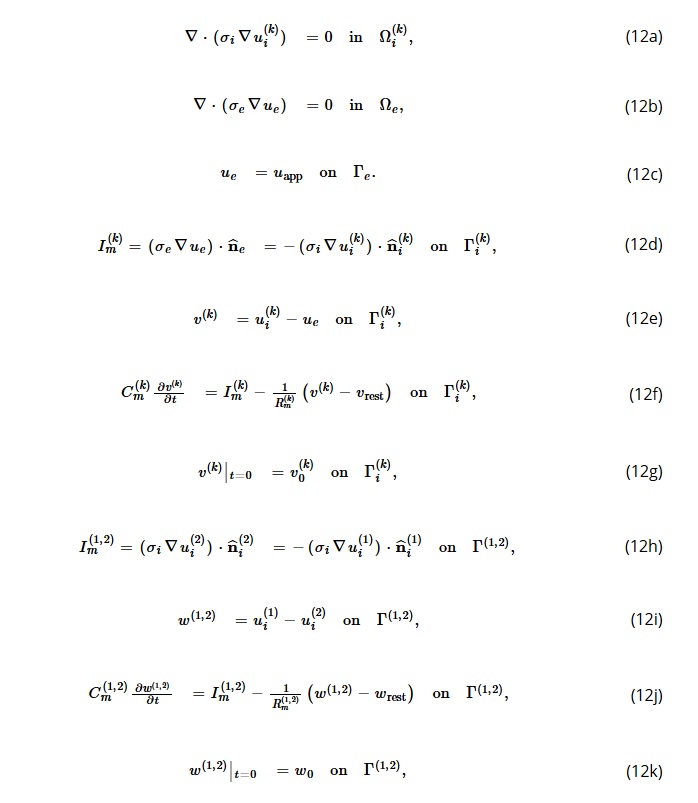
Actually, these equations aren't that hard. They mostly represent basic physical laws. It's the geometry that makes them interesting, and the good news is that meshes actually simplify the calculations. Clearly though, solving a dozen simultaneous equations takes longer than solving just one (you can see why people used to do this on supercomputers, and how parallelization can speed things up). To understand what these formulas mean, we have to back all the way up to the McCulloch-Pitts days, and the Perceptron (and its cousins Adaline and Madaline). With a binary neuron, the output is either 0 or 1, and when performing the synaptic calculations the concept of "resting potential" is non-sensical. Resting potential is always 0 for a binary neuron. What happens if we want a more realistic neuron, with a resting potential near -70 mV and a peak excursion of +30 mV during an action potential? In that case, all the carefully constructed weights we used to make the binary simulation work, go out the window - we have to recalculate everything based on the new voltage levels. What about if we wanted to model synaptic delays? In the Perceptron days delays were counted by ticks off the master clock, so if you told the Perceptron you have a synaptic delay of 2 ticks, it would keep the firing information around for 2 ticks and apply it at the right time. At any given time the machine had a "firing list" somewhere, consisting of all the neurons that had fired but not yet been applied. With a mesh, these conditions abstract in simple terms: there is a state before the calculation, and a state after the calculation. Everything is local, there is no concept of an artificial delay. If you have a neuron with a very long axon, and it has a detailed mesh around the hillock where the channels are, the easy way to save the CPU some cycles is by decreasing the mesh resolution in the areas where you don't need it. You may need it around the hillock, but you may not need it in some of the long cylindrical axon segments. The point being, you don't need a "regular" mesh. You don't need volume elements that are absolutely identical. However the equations above are framed in such a way that the symmetry simplifies the calculations. In a fluid dynamics simulation we're interested in the movement of calcium ions into and out of compartments, and with electric charge we're interested in the same thing, so in addition to conservation of mass and momentum we need to add conservation of charge. Fortunately, there are many excellent methods for describing the influence of external fields on local geometry, and we can use them to calculate the influence of a mesh cube on its neighbors. Right off the bat then, we have to focus on the boundaries, both boundaries that abut like astrocytes and synapses, and boundaries that partition, like endoplasmic reticulum.
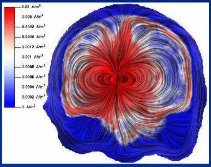
Here's a different kind of boundary. Here's a magnetic field in the brain. In volume conductor theory, the resistance of the extracellular fluid is much less than that of the bony tissue around the skull, so when the fields hit the skull they go laterally. (Which makes them harder to detect on the surface).
We can apply exactly the same principles to a single axon:
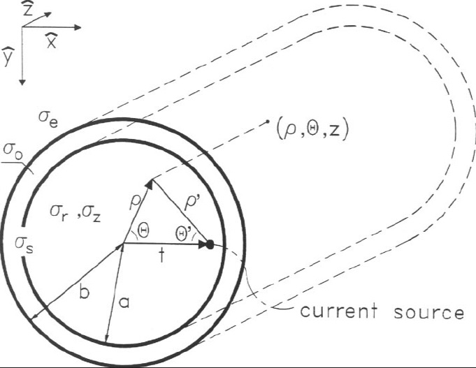
Generally when modeling the interactions of fields with charged particles (in fluids or otherwise) we will have:
- Equations of state
- Equations of motion
- Continuity equations
In our case this framework will include Maxwell's equations, and these equations all have to be solved at the same time, and in the general case they're nonlinear and computationally intensive. The tradeoff is, that any time we make compromises in favor of computation time, we're also compromising the accuracy and realism of the model. Meshes help us by simplifying the computational process. For example if we need to calculate a Laplacian we can use Stokes' Law to work around the boundary instead of integrating over the volume, and in a properly structured mesh, working around the boundary of a cell is a trivial exercise. Similarly, the derivative of a vector becomes the difference between its end points. For irregularly shaped cells we can calculate a metric tensor, which is just a matrix multiplication. The most frequent compromise made in these situations is attempting to eliminate the nonlinear terms in Navier-Stokes, and we can calculate how significant this compromise is, or simply compare simulation results. In a real brain the Reynolds numbers are low, there is little to no turbulence other than tiny edge effects, and most of the flow is laminar in the classical sense. CSF enters the brain in a set of channels that parallel the vasculature, it's almost all water (with very few proteins). It "perfuses" through the extracellular space, pulsating slightly with small pressure waves that mirror blood flow. In the tiny spaces associated with astrocyte leaflets the molecular composition becomes dense, the viscosity becomes high and charge effects become important, more important even than the fluid dynamics.
Let's look at it another way. There are hundreds upon hundreds of types of ion channels in a human body. There are over 300 types in the inner ear alone. A few dozen of these, constitute what we might ordinarily find in a human brain. But this belies the complexity of what we can do with these things, because the detailed placement of channels affects neuron behavior. As a simple example, the action potential can travel in any direction away from the point of generation. In some neurons, it travels antidromically (backwards) up the dendritic tree, at the same time it's being propagaged down the axon. What are the channel configurations that either support or prevent this behavior? If I need a unidirectional axon, how can I get it? Can I control the direction in which a signal propagates? These are good questions, and some of them have answers, but in general the full power of neural engineering has yet to be acheived, because there's no convenient way of wiring the circuit. With electronic components, you can wire up your circuit in a simulator like SPICE, and verify that it works "in theory" before you go spending money at the electronics store. In neuroscience, this order is often backwards, one has to sacrifice the animal before one can model its neurons. Today we know "enough" to be able to start wiring circuits in the simulator, however the simulator technology is WAY behind. You can take a look at SPICE, if you're an electronics person you'll understand what they had to do to make that work. Every different kind of vacuum tube has a representation that matches its I-V curves, if you tell SPICE you have a 12AX7 vacuum tube it'll know exactly how to model it. The same principle applies with the components of neural networks. If I tell Annie I have an IAF neuron, she has to know what it is. And fortunately she does, because if I tell her to calculate IAF's on a mesh she'll laugh at me (by giving me a lengthy set of error messages). The principle of a neural mesh is there is not just "one" membrane potential, there are many. Each element of a mesh has computations attached to it. Computing the mesh is very much like calculating the currents in an electronic circuit, one has to obey Kirchoff's Laws and ensure that currents and voltages are properly oriented. The principal side effect of a mesh is that point objects are no longer isolated. The whole idea of a set of synapses summing "into" a cell body is debatably non-biological. Things don't often work that way in real brains. Instead, a pyramidal neuron in the cerebral cortex has a dendritic surface upon which are embedded many "generators", in the form of spiny synapses. The surface is a membrane, it's likely a tightly stretched drum head. At the other end of the surface is a configuration of a different kind of generator, a set of channels that generate one or more action potentials. The exact interaction between one generator and another, is amazingly variable, it's nowhere near as simple as Hodgkin and Huxley's giant squid axon. An example has already been given - combinations of ion channels that generate subthreshold membrane oscillations, which can be found all over the brain, at widely varying frequencies but often in the 200 Hz range. Microtubules have a resonance in the 40 Hz range, and they're attached to the same cytoskeleton that houses the ion channels (and their voltage gates and ligand actuators). Since we already know that phase encoding plays a key information-carrying role in central brain circuits, it makes a lot of sense to look for ways of controlling the timing of action potentials. This is a complex topic, it would take pages of text to do justice to it. The short story is, one can "engineer" the shapes of neural responses, by constructing the appropriate geometries, of ion channels and the membrane itself. What if, say, I needed a biphasic response, the first part of which contains the location of the major inputs and the second part of which contains details around those locations? A question like this becomes more meaningful when framed in terms of information geometry. How are "multiple choices" represented in a neural network? In other words, a network or a machine can learn to discriminate between "table" and "chair" on the basis of a picture. What happens when I show it a picture of a table "and" a chair? Does it give me two outputs, or just one? Does it alternate between the outputs like a dynamic attractor, chair-table-chair-table, or does it somehow give me both "subspaces" of the answer in some kind of spatially encoded form? (Your chair info is over here, your table info is over there)? What types of networks can I build, to deliver the answer in one form or another? (Both forms apparently exist in the human brain).
The questions get broader when we consider what a neuron actually is. It's a cell - with a nucleus, mitochondria, endoplasmic reticulum, ... all these parts, have membrane potentials. The potential across the inner mitochondrial membrane is typically much larger than that of a neuron, it may be in the -150 to -180 mV range, and mostly that has to do with the protons that get created during ATP production (pH, is another way of looking at it). Endoplasmic reticulum also has a membrane potential, it's typically smaller but it becomes significant when we consider the relationship with calcium. Calcium is the currency of astrocytes, and there are several important types of calcium activity that play into neurons, including voltage gated calcium channels in the dendritic membrane, and waves of calcium activity in astrocytes that may be localized to very small segments of the leaflets initially, but if they escape they can turn into network-wide calcium storms dependent at least in part on gap junctions between neighboring astrocytes. Such a calcium storm directly affects the neural pathway from the entorhinal cortex to hippocampal CA2, which makes it important for everything from navigation to social learning. Whenever a neuron fires, there is a change in membrane potential that can trigger a myriad of intracellular effects, only some of which involve actual electric charge. Sometimes, the charge is ancillary to what's really going on, for example in the endoplasmic reticulum of cortical astrocytes there are IP3 receptors that amplify a calcium-driven calcium response. One of the distinguishing features of these receptors is that they are clustered, and the clusters have distinct spatial patterns along the surface of the astrocyte membrane. This is computationally significant, as shown very clearly by the machine learning models of Krotov and Hopfield. What happens is, the astrocytes endow a neural network with extra memory capacity and extra computational capacity, by adding higher order terms to the energy function, as shown in the figure.
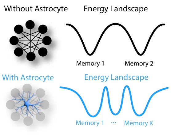
(Figure from Kozachkov et al 2024)
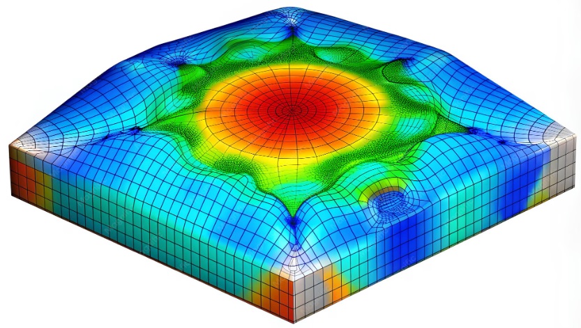
To merge the computational ideas of a geometric mesh with an associative memory (like a Hopfield network with astrocytes, which was recently studied by Dimitry Krotov while he was at IBM), we first have to understand what makes an associative memory "dense". More memories can be stored in an associative network by essentially making the mesh nonlinear, this way one can add maxima and minima "between" the vertices using polynomials and other interesting functions. The particular leaflet structure of cortical astrocytes makes them highly non-linear, in a very special way. The astrocyte itself is somewhat linear, it's I-V curve at the somatic level is almost a straight line in the absence of any special events. However the leaflets of an astrocyte process at least two different kinds of dendritic spikes, and even though astrocytes aren't known to generate action potentials, the transmission of calcium through the leaflets turns out to be highly irregular and non-linear. The peculiar distribution of certain astrocytes within the cortical neuropil points to an entirely different mode of integration in the apical tufts, one that's very local and involves only a few neighboring synapses ("neighboring" being defined relative to the astrocyte). And, the behavior of a neural branch is highly variable and depends on both the geometry (diameters and angles) and the configuration of ion channels. So if we wish to build a mesh that represents this situation, it won't be a simple set of cubes, because the astrocyte leaflets aren't built that way. The boundary at the outer edge of the astrocyte membrane will have the jaggies, and it'll be connected to things on the inside - therefore our mesh has to be treated in a special way relative to existing software. Here's a nice (irregular) finite element mesh that's perfectly suitable for computing the local potential around an ion channel. It's fundamentally no different from the square sheet of neurons shown above, except that it has some curvature and a thickness. And the things we calculate on this mesh are the same things we calculate in the traditional simulators, except that we call them something different. The ion concentrations we study are abstracted away as "membrane potential" in some simulators, which sometimes complicates the calculations by lumping a bunch of divergent variables into the same symbol. Neuroscience is intuitive, if you have four subunits in an ion channel you'll probably have a fourth order factor somewhere in your equations. The difference between an IAF neuron that doesn't account for this, and a Hodgkin-Huxley neuron that does, is enormous. The behavior of these neurons in populations is very different. The same principle applies at the level of membrane patches. The grid shown here, becomes part of a bigger grid when the whole neuron is considered, and that becomes part of an even bigger grid when the whole network is considered.
Here's the voltage dependendent ion channel that goes into the center of this mesh:
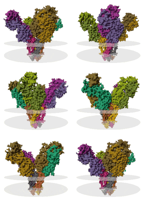
The two discs are approximately the extra- and intra-cellular faces of the lipid bilayer. You can see the large funnel-shaped structure on the extracellular side, filled with charged residues that attract cations. And, there is the narrow channel in the middle with a specific size and shape that makes it relatively selective for potassium (in this case). A voltage dependent channel typically has an arm that delivers a conformation change in response to changes in transmembrane potential, and an ion channel may bind with additional subunits that modulate its behavior, and sometimes these can be ligand gated or affected by intracellular messengers. These channels exist for sodium, potassium, chloride, and many other ions. In Hodgkin and Huxley's giant squid axon there were about 50-60 voltage dependent sodium channels per square micron of membrane surface, and slightly fewer than 20 potassium channels in the same area.
To drive home the issue of biophysics, we can observe that the Nernst equation originated in the world of chemical electrolytes. In the Nernst model, the formulas governing membrane potential are based on ratios, not absolute concentrations. However the recent data on ephaptic interactions demonstrates a significant effect of extracellular fields on neuron behavior. Sometimes the membrane potential can change by as much as half a mV as a result of a nearby axon firing, and this reflects the action of extracellular fields. Fields can act directly on ions, and they can also act indirectly on channel conformations. To understand the effects of extracellular fields near criticality, we need to take the biophysics into account. To put it bluntly, the connectionist model is simply inadequate in this case. The model below, is a starting point, but at the end of the day it's a grossly oversimplified version of what really happens.
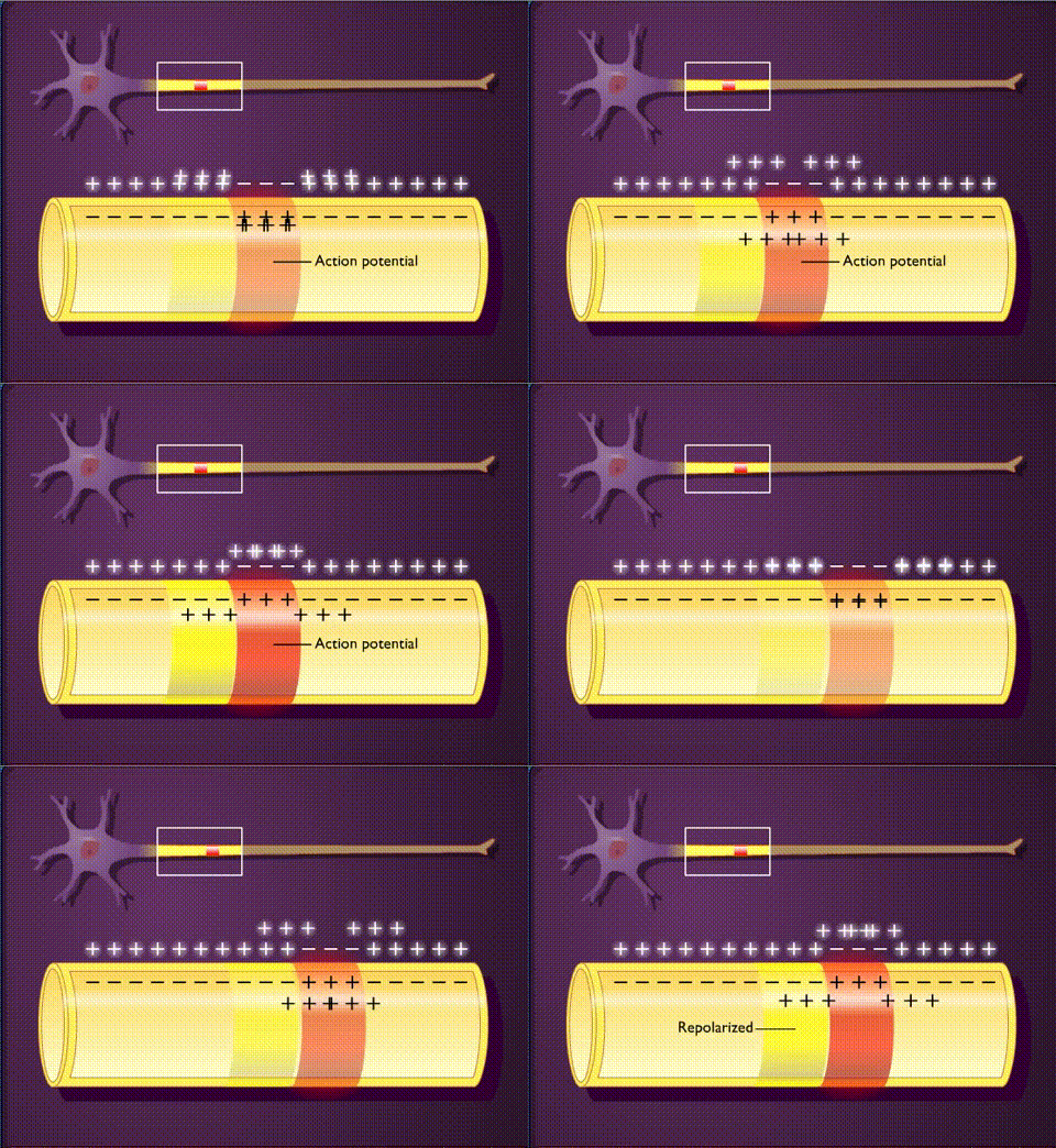
Here, there's an intracellular space, an extracellular space, and a membrane between them. The membrane has some kind of geometry, in this case it's a simple cylinder but in the more general case it'll be a mesh with an arbitary shape. We have ions on the inside, and ions on the outside, and they have different concentrations determined by movements laterally and across the membrane. Some of these are "leaks" and others are actively voltage dependent. In any given volume (inside or out), we have currents determined by the ion flows. As an initial approximation we can guesstimate that the orientation of the ion channels is normal to the plane of the membrane, so when a channel opens and ions rush in, they thereafter diffuse locally. Here is another representation of the same concept, with a traditional flavor along the lines of Rall's cable model. This time, we're getting closer to a mesh, we have regular computational compartments that can be solved locally.
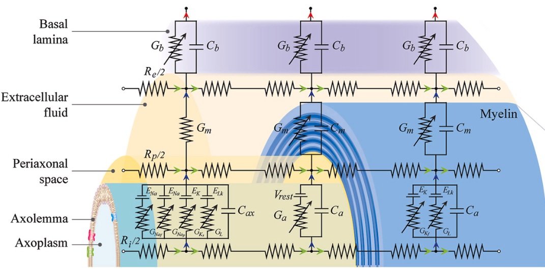
(figure from RaviChandran et al 2023)
This abstract mesh is "not bad". With this mesh, the authors were able to predict the effect of transcutaneous stimulation on a myelinated nerve bundle.
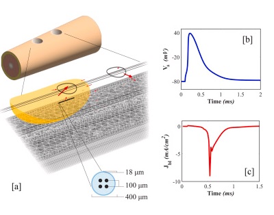
However a myelinated nerve is peculiar, the tightly wrapped glial membranes tend to diffuse currents laterally towards the nodes, and cerebral astrocytes frequently extend processes that connect with the nodes. An unmyelinated nerve is expected to respond more substantially to extracellular fields, because of the direct exposure to field (voltage) sensitive channels. Nevertheless this is an important advance and it's quite recent, and it lends itself well to ANNIE's modeling framework.
The authors at the top of the page used this same approach to look at deep brain stimulation. By now it is well known that extracellular electric fields can affect neural behavior at many different levels. This influence happens in the same way as action potentials, through ion currents both laterally and across the membrane. The electric fields across nerve membranes are enormous, million of volts per meter, but that's only because the membranes are so thin. The number of ions flowing across the membrane during an action potential can be quite small, and on the other hand leak currents can be large, involving a million ions per second through a single channel. (That's one ion per microsecond). How quickly do ion concentrations equilibrate in water? Well, that's an interesting question. Movement is restricted in the intracellular space. The intracellular space is almost like a gel, it consists of a thick network of cytoskeleton, endoplasmic reticulum, mitochondria, vesicles, and a host of other internal structures that take up space. And this is one of the interesting things about traditional models, they tend to treat the extracellular space as being free and easily navigable, while that is almost never the case in real brains. In real brains, the extracellular space is very tight. There's even very little water in it. The space between neurons is filled with glial cells, and nerve fibers in transit, and synapses on dendritic spines, and perisynaptic scaffolding, and all manner of cluttered geometry. Treating the extracellular space like an ocean full of sea water is a bad assumption.
So, more math. In neurophysiology, the Nernst equation gives us the equilibrium membrane potential based on the concentrations of ions inside and outside the cell:
V ≈ 58 mV * log (Cout/Cin)
for a monovalent cation at room temperature. However we have to step back a bit to understand the behavior of these ions. The Nernst equation describes the behavior of electrolytes across a barrier. In an electrolyte cell, the barrier could be a piece of filter paper, whereas in a neuron, it's a lipid bilayer. There is a concentration gradient across the barrier, and there is also an electric field, and the ions respond to both. If there were no electric field and no sodium pump, and if the ions could diffuse freely across the cell membrane, the concentrations inside and outside the cell would be equal and there would be no trans-membrane potential. In this case, the ion flux is related to the diffusivity of the electrolytes (ions) in solution, and it turns out in this case that the diffusivity of sodium, potassium, and chloride in native seawater is pretty similar, hovering around 10-5 cm2/sec, and this in turn generates fluxes in the volume elements inside and outside the neuron. The average of these fluxes, over time and over space, is 0 under equilibrium conditions. In the Euler/LaGrange and Navier-Stokes formulations, there is conservation of mass, momentum, and energy under several assumptions of uniformity, and unfortunately every one of these assumptions is violated in neurons. In a Hodgkin-Huxley neuron, a trans-membrane protein uses an ATP molecule to pump sodium out of the cell, or exchange three sodium ions inside the cell for two potassium ions outside the cell (causing a net efflux of sodium). This creates a trans-membrane potential, which in turn causes further rearrangements of the ions. There are additional ion channels in the membrane, including a passive potassium channel which then allows the K+ ions to rearrange themselves according to concentration and potential gradients. Additional there is a chloride flux, which is interesting because the chloride equilibrium potential is very close to the neuron's resting potential. Clearly, the nerve membrane has to be treated as a "barrier", that is to say, a boundary. The concentrations and potentials on one side of the boundary, are quite different from those on the other. The minute we start talking about astrocytes wrapping tiny feet around dendrites and synapses, the assumptions of uniformity go out the window. Astrocytes and neurons are often linked by specialized junctions, and extracellular scaffolding. The relationship between neurons and astrocytes seems to be very local. The active zones in glutamate synapses are very small, typically 10's of nm in extent. There are only a few ion channels associated with them. The vesicular release of transmitters is such that the probability is reasonably high that the opening of channels in an active zone is synchronized. Thus the impact of vesicular release is like a "pulse", and this takes us directly to the control systems view where we're interested in the steady state behavior and the impulse behavior.
In a small patch of membrane, then, we have a set of coupled equations. On the one hand we have the GHK equations that specify the membrane potential on the basis of ion concentrations, and on the other hand we have the Einstein-Nernst formalism that relates ion concentrations to membrane potential through diffusion. At the boundary, we have carefully controlled movement of ions from one compartment to another. Some things about this picture are obvious, like the forces associated with concentration and potential gradients. However other issues become thorny. Diffusion is contrained by the electric field, the diffusion "constant" actually becomes a tensor. The conservation of energy has to be calculated against ATP utilization, which is an independent variable and yet another important concentration (ATP is also a charged molecule!). We'd like a mechanistic model rather than a phenomenological model, but the more precise we get, the more it costs us in terms of computation time. It looks very much like we have to bite the bullet and just do it, because there's no other way. We're going to have to accept the reality of an hour per frame, and just slog through it as we descend to the level of the astrocyte foot and then ascend back up to the impact on spike times in populations. Consider for example, the concept presented in the mesh above:
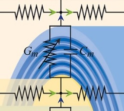
We can easily turn this into a mesh along the cylinder, which is the concept presented by the authors. The conductance Gm changes when we insert a channel into the membrane, as represented in this other piece of the authors' mesh:
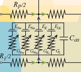
Great, this looks pretty close to GHK for a patch of membrane. Visualizing it this way, shows us some important features. First, the membrane capacitance is fixed. In other words, the time constants related to the opening and closing of channels can only be adjusted by changing the conductances Gx. Which is backwards from the way it actually happens - the actual time constant comes from the dynamics of the conformational changes in the protein channels, which "kind of looks like a capacitance" when we're just measuring membrane potential. The capacitance is physical, it comes from ion movement, which is to say current. There is an electrogenic component, and another component that isn't voltage sensitive. A careful perusal of the literature (since 1960 or so) reveals many many "simplifying" assumptions, and in the resulting simulation, these represent another way of "programming the results", as we discussed earlier. Nevertheless, this concept of "meshing a GHK equation" is still industry standard at this point. And, the dilemma of exactly "how" to model what we're seeing is a persistent plague, we simply have to try different things to find a representation that actually makes sense in the physical world. Looking at a colored mesh of your membrane potential is deceiving, because it's pretty. "Look ma, it works!" Well... not to belittle the accomplishment, but is it really telling us what we need to know? The meshes above were used to model a long bundle of nerve fibers with regular geometry, and they work in this capacity, but this is a very different scenario from looking at astrocytes wrapping a small piece of dendrite. The astrocyte contacts the dendrite only over a small region of the mesh, and within that region we would like a detailed mesh that allows us to use both GHK-type models and statistical models so we can see how they match up.
Channel densities directly determine the behaviors of small patches of nerve membrane. In the case of astrocytes modulating neuron behavior, we're specifically interested in the possibility of altering the spike timing, perhaps by shifting its phase by a few microseconds in either direction. Another piece of complexity is that ions interact, with themselves and with water, both inside and outside the cell. The intracellular milieu is viscous, almost gel-like, and the extracellular milieu can be quite similar in tight spaces, where diffusion is difficult. The space between an astrocyte and a neuron is definitely not uniform. It's thin, it consists of a tiny layer of water sandwiched between two lipid bilayers with large charged molecules sticking up out of them. Furthermore, ions like magnesium are small and highly charged and carry around "hydration shells" of water molecules with them. So when we're talking about a "diffusion coefficient" D, we're lumping together the effects of a whole bunch of separable phenomena. Maybe that's okay, it's probably fair to make a few reasonable assumptions at the molecular level. However the takeaway is, when we're looking at astrocyte processes that are only 50 nm big, we're almost at the molecular level. At that scale, molecules matter. Hydration shells matter. The competition between ions for space in a channel matters. Meshes are the only way to account for the geometry, and when it comes to neural networks, geometry is just about everything. The electrical activity depends directly on the geometry, all the way down to the atomic level, and all the way up to neurons in populations. To scale across these levels, we need computational meshes. The Nernst equation derives from the chemistry of electrolytes, and it works as long as the concentrations are uniform. In a neuron, the concentrations are never uniform. For instance the concentrations will be quite different in the middle of a 100 nm synaptic active zone than at the ends. Therefore our mesh has to treat the local ion concentration as a variable, and derive the membrane potential from it, rather than the other way around. (That's a glaring problem with IAF neurons, you have to declare the resting potential!)
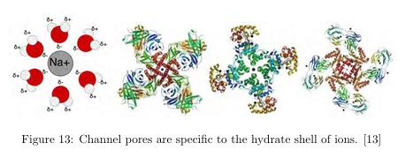
(figure from bernstein-network.de)
To develop this theme further we'd have to get into some detailed math, and we probably don't want to do that just yet. The principled description above should be sufficient to understand the issues. These issues provide us with a very important and challenging requirement when it comes to our workflows: we need the ability to quickly and seamlessly heal and join meshes of all different sizes, shapes, and densities. When we're at the synaptic level, or the level of astrocytes wrapping dendrites, we need very fine meshes. When we're at the level of Nodes of Ranvier, we can get away with coarser meshes if we're just interested in signal propagation. If we want to look at the resulting spike trains in the populations of thousands of these neurons, we need the ability to zoom out and visualize the relationship between the zoomed-out view at the population level, and the zoomed-in view at the synaptic level. And this is a vital concept when it comes to computational meshes: the first step in every simulation is the acheivement of a perfect computational mesh. Perfect has several meanings. In the sense of differential geometry it means our mesh wants to be "manifold", it doesn't have any holes, or discontinuities, or nasty edges. In the sense of a computer data structure, the mesh has to be rapidly transformable, because the operations required to achieve a perfect computational mesh involve repeated decimation and restructuring, and it's an interactive process, one has to be able to look at the results on-screen in real time. Another sense of perfection is the ability to attach data structures to the objects in the mesh. Generally we will have sub-meshes within a larger mesh, for example endoplasmic reticulum within a cell body or a dendrite. There has to be a robust and air-tight set of algorithms to identify and maintain "objects" as we change mesh resolutions and move things around. And of course, we don't want to be tracing every ion channel from pictures, so we need ways of "populating" the mesh, with channels, with synapses, with neurons, at all different levels of resolution - and that means we need collision detection and a whole bunch of other "validation" algorithms to make sure our mesh will support the computations we need. However the basic concept is the same at all levels of resolution, and it's been time tested and field tested for over a hundred years. We want named objects positioned in space with data and functions attached to them, addressable in some kind of scalable coordinate system. Such an implementation will allow us to move seamlessly between different representations of the same objects, for example the concept of vertices with varying distance is different from the concept of voxels (as used in, say, medical imaging). In some cases it helps us to have a voxel based representation, in some cases the unstructured mesh is preferred, and in some the cases a sampled point cloud is advantageous. These are more than just visualizations, the way the geometry is handled determines in large part the way the computations have to be handled. For example the faces of a mesh can be treated as differential 2-forms, and if we need to use them this way, a half-edge data structure at the level of the edges helps us navigate the vertices. These figures could be little bits of endoplasmic reticulum in a volume of neuron or astrocyte.
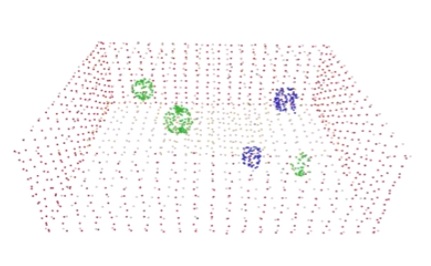 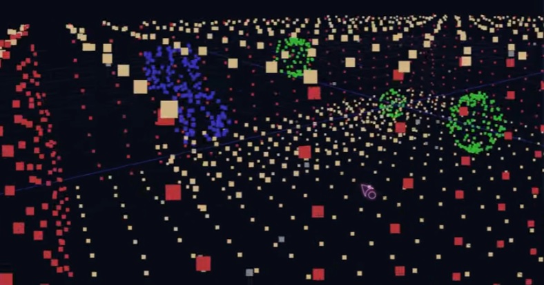
(A sampled point cloud and some voxelized 2-forms: Open3D examples by Florent Poux)
That being said, Annie's purpose is to make computational modeling easy, and meshes are the answer to a lot of the problems that plague computational neuroscience today. Including the many ways it overlaps with machine learning, like predictive coding for example. Neuroscience as a discipline hasn't even begun to explore the richness of neuronal dynamics yet. Since the seminal paper by Wilson and Cowan in 1972, there has been some effort in the area of volume conduction but it's only recently that the concept of topographical dynamics has gained traction (in the form of dynamic neural attractors and other such elementary concepts). For me, that's a big duh! I started in neuroscience in 1978, before the Hopfield network. Back then, the biggest thing was Kunihiko Fukushima's Neo-Cognitron, an early form of convolutional network. But quietly, at the same time, Shun-Ichi Amari was developing the foundations of information geometry, beginning from statistical neurodynamics. If life is fair, Dr. Amari will be the next Nobel prize winner. The thing is, the neuroscientists don't know what to do with his invention yet. (No diss, because neither do I!) We (as a group) have no idea how to get from neurons to information geometry. We do know however, that it involves astrocytes somehow. My hypothesis is that astrocytes regulate both the size and shape of the sharp wave ripples in the hippocampus. In other words, they guide and constrain the information geometry. There's only a few million neurons in the hippocampus, we should be able to model the whole thing all at once, and in fact people have tried, and some have even come pretty close. But only using traditional simulators, not with meshes. It seems reasonable to set a modest target of 100,000 neurons, a size that corresponds approximately with both the extent of an astrocyte and the extent of a sharp wave ripple. With 100,000 neurons in a meshed simulation, it should be possible to complete a computational tick within 10 seconds. With the C language version of Annie's server, this is possible. With Python, it's not possible because Python is interpreted and its lists are much slower than direct pointers. With Python one can expect exponential performance degredation as the lists grow. 100 meshed neurons will take 30 msec, 1000 neurons will take 3 sec, 10000 neurons will be a cup of coffee. However... these are some of the visualizations that result. These examples come from the MFEM project at the National Labs (Argonne, Sandia, Lawrence Livermore). They're professionals with finite elements, they've been doing it for a long time and neuroscience has a lot to learn from them.
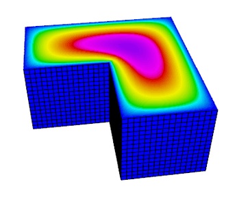 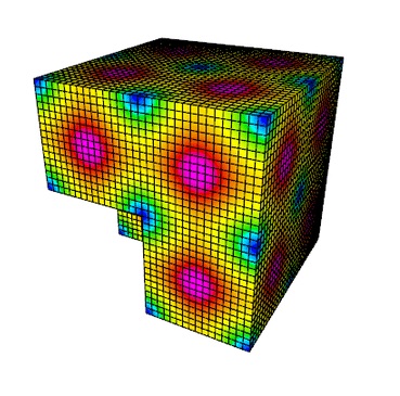
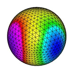 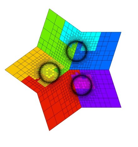
This one could be a usable starting point for an astrocyte model, you can see the micro-domains forming as the result of changing boundary conditions. The gradients could represent potential gradients. These are the types of visualizations that help us understand the problem domain and the range of solutions.
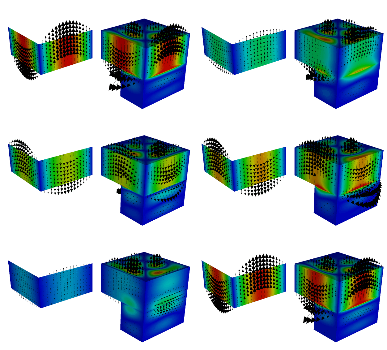
To get from a simple Hodgkin-Huxley neuron membrane to an animation like the above, we need the mesh to be in a certain form. Those of you who are familiar with the finite modeling landscape may have seen or used tools like Comsol, which is a very powerful simulator, and in the open-source world there is FEniCS, which is also powerful. However these computational engines are billed as "multi-physics", whereas Annie is pure neuroscience. Of course, neuroscience is physics too, but biophysics is a little weirder than structural mechanics because of the geometry. Nevertheless, the physics is the same, we must handle the charges, the fluid flow, and any mechanical distortions. Mechanical distortions become significant in neurons and astrocytes because of the cytoskeleton, which is often rich in highly motile actin fibers. "Neurons twitch", as they say - and so do astrocytes. In the case of astrocytes, the mechanical lability is strongly associated with synaptic determination (growth and pruning). Some synapses don't form at all without their astrocytes. From the standpoint of cell biology and neuroscience, one can be absolutely certain that the relationship between neurons and astrocytes is considerably more intricate than just nutrition. The clusters of IP3 receptors are involved in generating the astrocytic phenomenon known as "calcium puffs", which are localized and directional. It is very likely that it's these puffs that end up affecting the neural dynamics, and when the puffs become big enough they can turn into network-wide calcium events - which curiously enough have a longer time course than the firing of neurons, an astrocyte storm lasts for several hundred milliseconds (which might encompass several cycles of theta).
The critical brain hypothesis requires us to take the issue of spike timing seriously. In theory, the opening of a single ion channel (or lack thereof) can affect membrane behavior. When the neuron is near threshold, it requires "enough" of the right ion configurations to generate an action potential. "Enough" is hard to quantify. How many ion channels are involved in a visible subthreshold membrane oscillation? Well, to see such a thing, you have to measure it, and to measure it, the usual way is to put an electrode somewhere. You can't isolate a few ion channels with an electrode, so how are you going to determine the shape of a membrane oscillation? 2-photon calcium imaging? Good luck! Sometimes, subthreshold oscillation only becomes visible in response to (synaptic) input, which means it must be very local, involving only a few channels. The number of ligand-gated channels in a synapse is variously quoted to be pretty small, around 10,000 or less, with 100 or 1000 channels in an active zone. So why would a synapse need oscillations? Well, the obvious answer is that the oscillations will either amplify or diminish the effect of subsequent inputs, depending on their precise timing. These are small oscillations, but they matter when the neuron is near threshold. Near threshold, a small oscillation can either advance or delay the action potential. This behavior is well known in control systems theory, as it relates to ringing filters, which affect the stability of the system and therefore become important in the consideration of dynamic attractors. The bottom line is we need simulators that will show us the precise behavior of a neural network under carefully controlled conditions. From the standpoint of free energy and criticality, we need to be able to visualize the boundaries of critical regions, because that's where the theory tells us we should find the fractal behavior and power law dynamics. Looking at one neuron is not enough, we need to see the population, and each neuron has to be sufficiently detailed to show us real behavior (like the dynamics of transient oscillations). The entirety of the field of neuroscience is heading in this direction, a few years ago people realized that biophysics is a rigorous discipline and toy simulators aren't going to help much. The things that help, are visualizations like the potassium channel. One look is intuitive, you can see how it works just by looking at it.
Annie was born from need, I'm using her because I need her. There's no other tool that can provide the simple geometry needed to test a novel idea. A while back I needed a transverse Hopfield network, and no one could give me one. Not TensorFlow, not Brian2, not Nest or NEURON or any of the others. Because none of them really understood geometry, their solid body skills were lacking. After all, how hard is it to rotate a few neurons around the Z axis? I find it hard to believe that no one has ever cared about this in the entire history of neuroscience. I rather guess that people got lazy and sacrificed accuracy in favor of publication time. Faced with the lack of a readily available solution, the only other option was to roll my own toolset from Python libraries, and as long as I'm doing all that work, might as well do it right. So other people can use it too - because at the end of the day we're all after the same thing. The chances of me becoming the next neuroscience Einstein are pretty small, so I'll just focus on the toolsets and build a nice usable environment for scientists, because I know how to do that. The human factors are important, we need reliable software and that was actually easier a few years ago before AI. Now there's an explosion of tools but most of them are buggy and aren't being adequately maintained. Even VTK is full of bugs, even after being field tested in the National Labs for 20 years. There's no way to exercise the full breadth of these powerful tools in testing, there are too many pathways and too many ways to use them. I end up fixing a lot of bugs in other peoples' code, it's an inevitable part of open source development. But achieving the goal is worth the pain. (No pain, no gain - as they say at the gym).
|