ANNIE Completes The Picture
The first and most essential piece of computational geometry is solid body modeling in three dimensions. Lately we've seen an explosion of results in AI-assisted connectomics, and this has created some wonderful visualizations, but there are some essential pieces missing. In the amazing reconstruction below from the MICrONS project, where are the astrocytes?
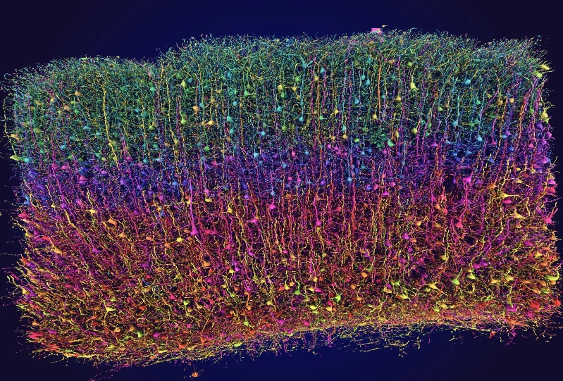
What about organelles? At a biophysical scale, we're certainly interested in things like mitochondria and endoplasmic reticulum. And reconstructions like the above don't represent internal membranes. If we try to compartmentalize a branching dendrite to get a more accurate view of the biophysics, we still have no way of accounting for the effects of external fields on the geometry. As neuroscience advances, it becomes important to quantify biophysical behavior at high resolution, and scale its effects across the entire brain. To move from algebraic simulators like TensorFlow and traditional differential simulators like NEURON, to full-blown biophysics, we have to invoke methods like FEM (finite element modeling), that allow us to do more than just manipulate ion concentrations. On this page we'll look at the traditional view of neural network simulation, and segue into a more modern view, showing the link between connectionist networks and biophysical geometry. If you work with neural network simulations, this will look familiar. On the next page we'll raise the bar a bit, but there's still an enormous number of existing workflows that use traditional models, and plenty of researchers who aren't yet acquainted with the new methods.
Overview of ANNIE's Work Flow
Annie's work flow converts traditional neural network models into full-blown multi-biophysical simulations. Here are five ways to begin with ANNIE:
- From a tracing
- From a microscope stack
- From synthetic geometry
- From a network definition file
- Interactively using the dashboard
ANNIE will first convert any geometry into the required three-dimensional representation. Traditional network geometry becomes discrete simplicial manifolds in a coordinate space. Once a perfect watertight and manifold mesh is achieved, ANNIE proceeds as follows:
- Partition the mesh into computational compartments
- Define the boundaries between compartments
- Assign physical materials to each compartment
- Define the computations on mesh elements
- Apply initial conditions to compartments and boundaries
- Export the entire structure as a finite element simulation
Once ANNIE has created a common intermediate format, the finite element construction is translated into a simplicial complex suitable for discrete simulation using the methods of differential geometry. In this form, ANNIE computes the full multi-physical spectrum including mechanics, charge, and fluid flow. ANNIE's output can be visualized in any convenient viewer (ParaView, VTK, PyVista) in any convenient form (STEP, BREP, CGNS, etc). ANNIE can save the entire simulation package in HDF5 form for easy cloud exchange.
ANNIE As A Traditional Neural Network Simulator
Let's start from the beginning. ANNIE has an extensive text mode. A while back, the assumption was you were going to load your simulation into the mainframe from a text file and come back in the morning when your results were ready. The parallel supercomputers shortened the wait time from overnight to an hour, but the simulation process was still viewed as a "job", it wasn't exactly interactive. Annie's original purpose was to create the computational meshes needed for accurate membrane modeling. Such an effort requires the detailed tweaking of parameters, and this is still often easier to accomplish with an editable text file rather than a form on a screen. So Annie provides the text capability that lets users define and maintain networks in simple and intuitive ways. There is interactive capability too (as shown), but let's talk about the text first, because it's a common denominator that will be recognizable no matter which discipline(s) you're familiar with.
Two of the hardest parts of a simulation are stimulus orchestration and data collection, and Annie makes them easy. When defining a simulation, you have to give it a name. The syntax is: SIMULATION < simulation_name >
Next you have to tell the simulation which network(s) to use, with one or more lines like the following: USE NETWORK RETINA
Templates are stimuli. Stimuli are geometric patterns with relative coordinates (relative to the base of the template). For example in the visual field, there are points of light, bars, circles, annuli, gratings, random dot stereograms, and so on. These stimuli can move, which is what an "Apply" directive defines, it defines how the template moves. The stimulus template is "applied" to a particular network object (a neuron, a synapse, a module, or an entire cell group). The syntax for applying external stimuli is:
APPLY TEMPLATE < template_name > TO < object_type > < object_name >
Templates are more than just geometric patterns, they can contain functions and modifiers. Templates are usually organized into files that can be loaded up front with one or more directives of the form LOAD_TEMPLATE_FILE < filename >. Within each template file are one or more template definitions. These are named. In the APPLY statement, you use the template name. Each APPLY statement has multiple directives that control the action of the template on the designated cell group. Template actions are additive, for example if you have two dim spots of light affecting the same cell, they will add together to form a larger response.
Here is an example of a complete simulation definition file. Any line that begins with an asterisk or a # is a comment.
SIMULATION RETINA_SIMULATION
* tell the simulation which network to use
USE NETWORK RETINA
* template names are defined in the template file
LOAD_TEMPLATE_FILE cones.tem
* apply a named template to a cell group
APPLY TEMPLATE T1 TO CELL LIGHT
STARTING_COORDS (-9000,-9000,1000)
MOVEMENT_COORDS (1000,1000,0)
SCALE (2,2,0)
START_TIME 0
STOP_TIME 120
INCR 2
LOOP 7
REPEAT FOREVER
The coordinates are defined relative to the network. The network coordinates form a "coordinate space" within which neurons are populated and within which templates are applied. Each template has a size and an orientation, that can be scaled and rotated as needed. The template primitives are combined to form more complex stimuli, for example gratings are combinations of bars. You can also use ordinary .JPG's if you wish. To use a template, simply declare it inside a template file. Here is a complete example of a template definition file, containing four stimuli with widely varying behavior:
TEMPLATE T1 SIZE (6000,6000,0)
BAR (0,0,0) TO (2000,1000,0) LEVEL 5.0
BAR (3000,3000,0) TO (5000,5000,0) LEVEL 5.0
TEMPLATE T2
* SIN(A,K,W,P)
POINT (9250,9000,0) FUNCTION SIN(10.0,0,10.0,0)
TEMPLATE T3
CIRCLE (4000,4000,0) DIAMETER 2000.0 LEVEL 5.0
TEMPLATE T4
ANNULUS (3000,3000,0) OD 2000.0 ID 1500.0 LEVEL 5.0 LEVEL_SCALE -1.0
The first example shows a pair of simple bars (one of which is a square). The second example shows the use of a function to determine the level (note there is no level directive here, the function sets the level). The last example shows a LEVEL_SCALE directive, making the annulus dark relative to the background. When this stimulus is applied, a value of -5.0 will be transferred to the target cell. Templates can be applied to just about anything, including external structures for volume conduction and field stimulation.
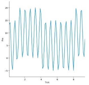
Here is the effect of template T2 (above) on a synapse. You can see the sine wave in action, and in this experiment a nearby slightly weaker grating of light is also affecting the synapse, you can see the modulation as it moves across the cell's receptive field. With templates, you can attach arbitrary functions to points in space and have them move over your grid.
Conversely, there is also a need to program spike trains, for example when one is studying the membrane behavior of a single neuron as it relates to synaptic input. ANNIE can create a wide variety of synthetic spike trains, with directives like INTERVAL, BURST, and POISSON, to provide a usable library of exploratory stimuli. Spatial patterns are most significant for topographic neural networks like the retina, whereas temporal patterns become important in phase encoded systems like the hippocampus. Annie provides a quick and easy way of manipulating both domains.
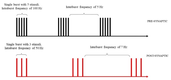
(Figure from Micheli, Ribeiro and Giorgetti 2021)
You can get stimuli into any part of Annie's models. You can apply them as patterns picked up by receptors (like light on the retina), and you can apply them directly as membrane potentials and indirectly through synaptic inputs. Typically in finite element and volume modeling we start with simple linear implementations that gradually get more complex as we begin to understand the boundary conditions, so we have a need to interact with the model at many different levels of sophistication. ANNIE provides the complete spectrum of stimulus application capabilities to support the entirety of these workflows. Later in these pages we'll see how ANNIE converts pixels to physical forces on tiny patches of membrane.
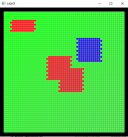
By the way, the graphics are highly interactive in a live ANNIE environment. ANNIE is certainly capable of traditional network visualizations, but raises the bar with analytics that can be overlaid onto the network structure. A time series of synaptic activity doesn't really help us understand receptive fields, what we really need to see is the pattern of activity in a cell group, relative to the stimulus input. Here is one of many ways Annie can visualize this for us. We can look at cells as a grid, even if they're not geometrically arranged that way, and if there's a topographic mapping we can see how the stimulus maps onto the network activity in real time.
 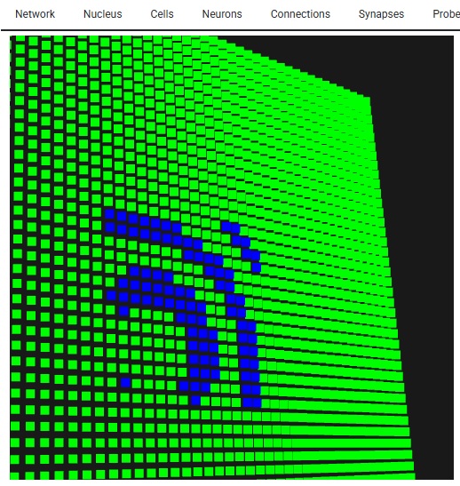
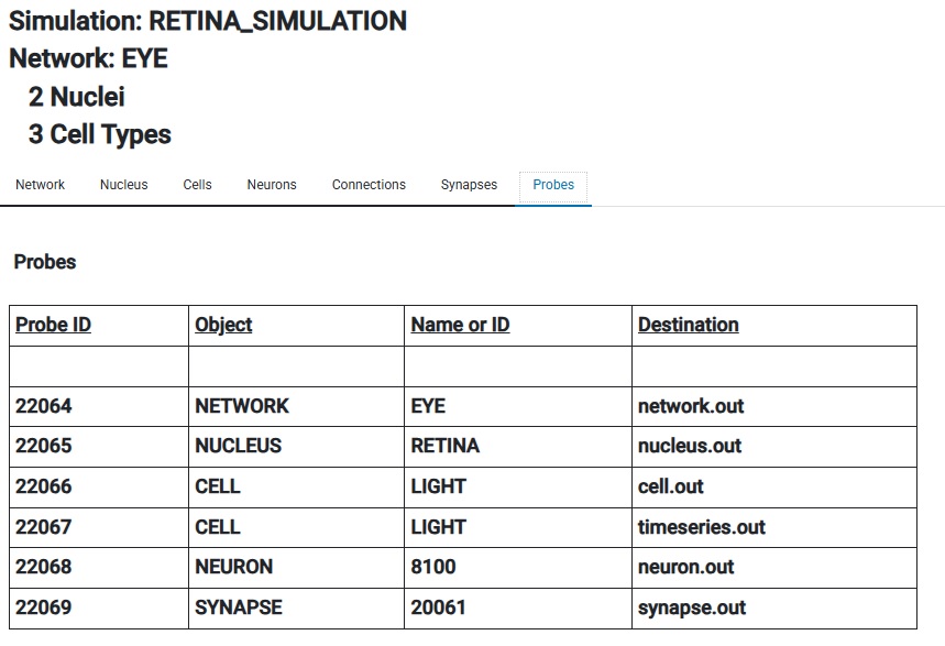
And of course you can still see information the old fashioned way too. Here are some "probes", which are ways of getting information out of Annie. Probes can export data in just about any format (CSV files are a staple, for direct import into Pandas, and Annie can export geometry in 30 different formats including the industry standard OBJ, PLY, and STL files, as well as the HDF5 format used by the cloud based systems). In a personal context, data files are the most common need, but in the full multiprocessing client-server version of Annie you might see entries on the right that say "Client 17 Window 5", and those would be real-time streams destined for a workstation. On the workstation side, probes can be visualized in many different ways, ranging from time series and spectra to spatial displays and correlation maps. Probe output can be overlaid on geometry for precise visualization of network activity.
ANNIE uses the same simple philosophy to define networks, organize them, and re-use them in sequences of experiments. No programming is required, only the ability to tell ANNIE what you need. A network can be as simple or as complex as you like. This is a valid network:
* no synapses here
CELL RODS N_NEURONS 100
This is another valid network:
* no cell group, just one neuron
NEURON NAME ABC TYPE IAF TAU 0.1
SYNAPSE FROM ABC TO ABC TYPE INHIBITORY WEIGHT 0.1
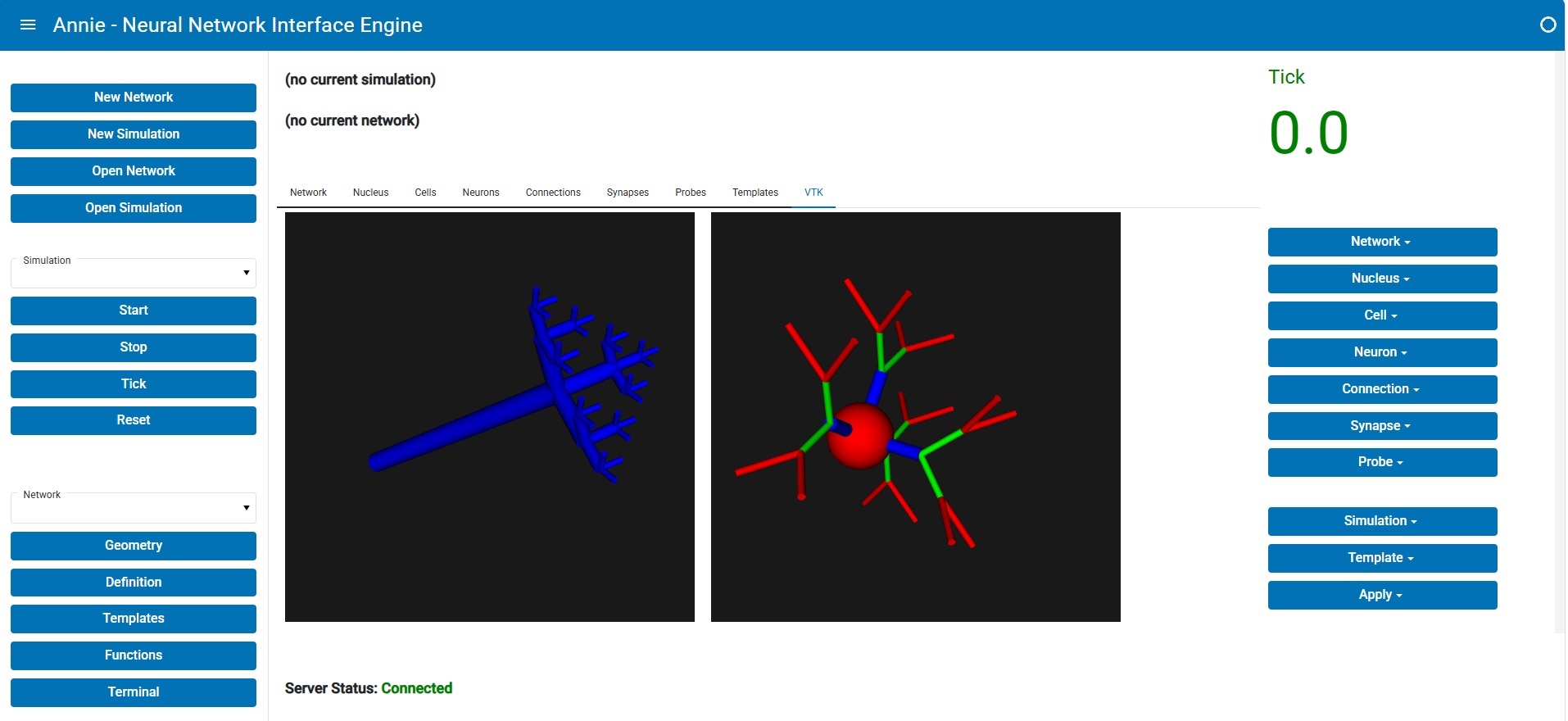
When you "Open Network" on the dashboard, you're reading in a network definition file. In the client-server version the build goes through stages, there is verification followed by downloading, but in ANNIE's standalone mode you can do the same thing interactively with a few mouse clicks, by saying "Create Network" instead, and then building the network at your own pace using the menu buttons on the right (ANNIE's dashboard is below). When you create a cell group this way, ANNIE will show you a complicated-looking form that you can fill in at an excruciating level of detail, or you can just push the "OK" button and accept the defaults. The defaults will always work, and Annie will let you know if there are any problems or conflicts.
Here is a slightly more detailed network definition:
NETWORK EYE
CENTER (0, 0, 0)
EXTENT (12000,12000,12000)
NUCLEUS RETINA
CENTER (0,0,6000)
EXTENT (10000,10000,2000)
ORIENTATION (0,0,1.5)
CELL RODS
CENTER (0,0,6300)
EXTENT (10000,10000,5)
N_NEURONS 40000
ARRANGEMENT GRID_2
In this example, we've defined a network coordinate space of (-12000,-12000,-12000) to (12000,12000,12000). ANNIE will check that everything we subsequently define lives within this space (the primary reason for this is to account for and control for edge effects). Within the network called "EYE", we've defined one nucleus called RETINA, and within that there is one cell type called RODS. (We don't have any synapses yet, we haven't defined any connections). You don't have to actually type these files, ANNIE will type them for you. You can build things interactively, and whenever you're ready you can save your network in an easily readable and editable form.
To take the network definition to the next level, we can specify the details of each neuron type, for example:
CELL RODS
CENTER (0,0,6300)
EXTENT (10000,10000,5)
# NEURON_SIZE (2,2,5) VARIANCE (0.1, 0.1, 0.5)
N_NEURONS 400
ARRANGEMENT GRID_2
# length and diameter are given in microns
NEURON_SHAPE CYLINDER LENGTH 5 DIAMETER 2
NEURON_TYPE PASSIVE
RESTING_POTENTIAL -50 VARIANCE 5
TAU 0.05
Here we've given our photoreceptors a cylindrical shape, and we've defined them to be passive with a resting potential of -50 +/- 3 mV. They're also fast, they have a 50 microsecond membrane time constant.
Creating connections is just as easy. Here are some examples:
CONNECTION < cname > FROM RODS TO BIPOLAR_CELLS
TYPE INHIBITORY
WEIGHT 0.1
TAU 0.05
TOPOGRAPHIC
DIVERGENCE 5
SYNAPSE FROM NEURON_A TO NEURON_B TYPE GAP_JUNCTION_43
PROJECTION FROM SN_PC TO STRIATUM
USE CONNECTION < c1 >
USE CONNECTION < c2 >
So far this looks a lot like a traditional simulator, right? With ANNIE you can easily define your network at the same level as a NEURON or a Brian2, using differential equations that mimic current flow in compartments with specific conductivities. If we've already defined this network somewhere else, like in NEURON or even TensorFlow, we can easily import it into ANNIE with two mouse clicks. But ANNIE does a lot more geometrically, than these connectionist engines. ANNIE creates global geometry that allows you to accurately place your cells within a network, and your network within a brain, and your brain within a skull, with high-resistance meninges and bony tissue and a microtrabecular network of vasculature immediately above the layer I axons in your model cortex. You'll notice the ORIENTATION keyword above. In the networks at the top of the page, the one on the left was given a pitch, and the one on the right was declared as a CLUSTER. Network definition is very easy with Annie, she's masterful with the solid body geometry and she'll make sure your network is geometrically correct and computable.
ANNIE can populate your cells from the specification above, and you can create neuron geometry the same simple way. You can create the Lego neurons shown below with directives of this form:
AXON CYLINDER ORIENTATION (10, 20, 20)
BRANCH 3 TIMES (10,10,10) LENGTH 5
And we'll look at several other ways of creating neurons on the next page. Don't be fooled, these neurons aren't toys. They are computational meshes, that resolve down to the nm range. Legos are only a starting point, as we'll see. ANNIE thinks like a neuroscientist, she allows you to define your network directly in terms of brain anatomy and physiology. She knows about nuclei, neuropils, modules, layers, and synaptic capsules. ANNIE has a sophisticated structural engine that creates axons and dendrites and properly inserts them into their geometries and connects them with their destinations. You don't have to provide ANNIE with connection maps, she already has them. If you have a topographic connection from one layer to the next, you can say DIVERGENCE 5 and you're done, ANNIE will connect each cell to its 5 nearest neighbors in the destination layer. No fuss, no muss.
ANNIE lets you design networks at a more sophisticated level than NEURON or TensorFlow. But this isn't enough, ANNIE's purpose is accurate biophysics. We have to transition from treating neurons as spheres with a few attached cylindrical compartments, to computational meshes with nanometer resolution. Even the Lego-style ball-and-stick models are hard to accomplish with many simulators, because traditional simulators tend to treat neurons and synapses as isolated entities, rather than open biophysical systems. Cable models, while more realistic than Perceptrons, don't account for mechanical forces and fluid dynamics. We'll take a closer look at some computational approaches on the next few pages. For now, it is noteworthy that astrocytes use different communications methods than neurons, the electrical signaling that occurs between astrocytes is for a different purposes and involves different mechanisms. Yet in real brains, neurons and astrocytes are only 20 nm apart from each other, so close that calcium ions have a hard time diffusing in the space between the membranes. These physical effects need to be accounted for. Calcium has a direct effect on the shape and physical properties of the cytoskeleton, which affects everything from the shape of dendritic spines to the wrappings of astrocyte leaflets around synapses.
From Neural Networks To Biophysics
Let's begin making the transition from traditional network models to multi-physics. The easiest way to understand this is in terms of geometry. In a connectionist network, sometimes we only need synaptic weights and neuronal threshold functions. But a biophysically realistic simulation requires us to perform calculations at the molecular level, or nearly so - and this is a different concept from compartmentalizing a cable model. We need the network-level description too, because without it we can't understand the biophysical results in context. And sometimes we even need more than that, maybe we want to look at the effects of trans-cranial brain stimulation on the astrocytes in the amygdala, so we need geometry for the angles of the field and the nerve membrane, and any other nearby structures that happen to contribute. ANNIE ties it all together. ANNIE scales over 8 orders of magnitude with 64-bit floating point math, and up to 12 orders of magnitude with 128-bit capability (which is currently provided only by supercomputers, unless you're willing to wait for the slow results from software emulation).
Using ANNIE, you can model neural networks as simple or as sophisticated as you wish. ANNIE will handle the cable models and the synthetic geometry as shown below, but the real purpose is to advance beyond these primitive models into realistic biophysics. The traditional views are available for transitional purposes. Using ANNIE one can create a completely automated workflow all the way from imperfect SWC tracings to computationally perfect 3-dimensional simulations that support multi-physics, including charge, mechanics, and fluid flow. An entire workflow can be accomplished in a few minutes when the right tools are available. One can begin with a low quality tracing, convert it to a watertight surface mesh, volumetrize the mesh and extrude it so it attaches to a cytoskeleton, partition the mesh into computational compartments, add internal organelles like mitochondria, specify physical properties for the various mesh elements, and place the entire structure inside a set of external fields controlled by dynamic stimulus templates. The traditional simulation structure serves an essential purpose in this framework, insofar as it allows us to visualize results in the same way we would see them in a live brain.
ANNIE can build networks quickly and efficiently. At this level ANNIE looks a lot like a NEURON or a Brian2, but she's friendlier and more powerful. ANNIE does everything in 3 dimensions, so if you'd like to visualize a sheet of neurons, you can rotate it and scale it interactively, view your activity levels from any angle you like. This is already a value-add, because visualization is important. How would one make sense of a network like the one shown at the top of the page? One would have to unravel it somehow, take density and distance measurements and try to reconstruct the wiring from pictures of the synapses. ANNIE can take the opposite approach. Earlier we mentioned synthetic geometry, and Lego neurons. Take a look at these simple synthetic neurons. Each of these were built with two lines of text in a definition file.
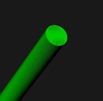
These shapes however, are considerably different from the ball-and-stick neurons discussed in the NEURON tutorials. They are actually very fine (computational) meshes, as you can see here. The axon below resolves to 1 nm. You can easily insert ion channels into the membrane at the locations of your choice. This is where ANNIE departs from the traditional simulators. To get this anywhere else, you'd have to jump through hoops. ANNIE does the translation from traditional network models to realistic multi-biophysical simulations. On this page we saw a network definition language that looks a lot like a NEURON script or some Python code for TensorFlow. On the next couple of pages we'll look at some different starting points, for both synthetic geometry and microscope images. As you can see here, ANNIE's resolution is better than any microscope image. The mesh for this axon is about the same size as a hydrated glutamate molecule. ANNIE can do even better. Given 128-bit computational support, ANNIE can resolve well beyond the range needed for Monte Carlo simulations associated with Brownian motion and molecular dynamics.
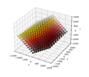
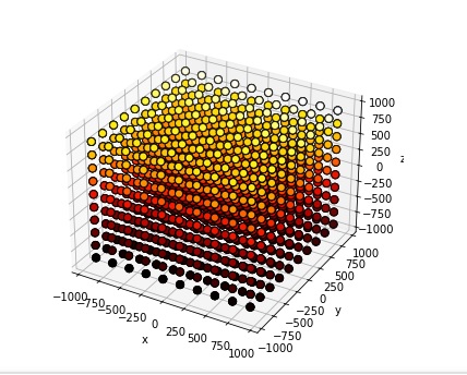
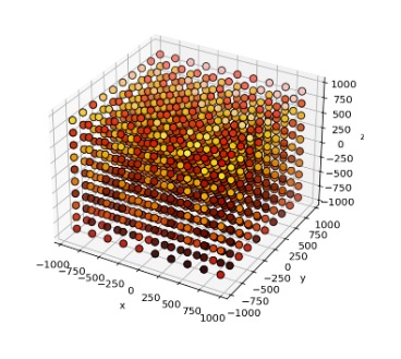
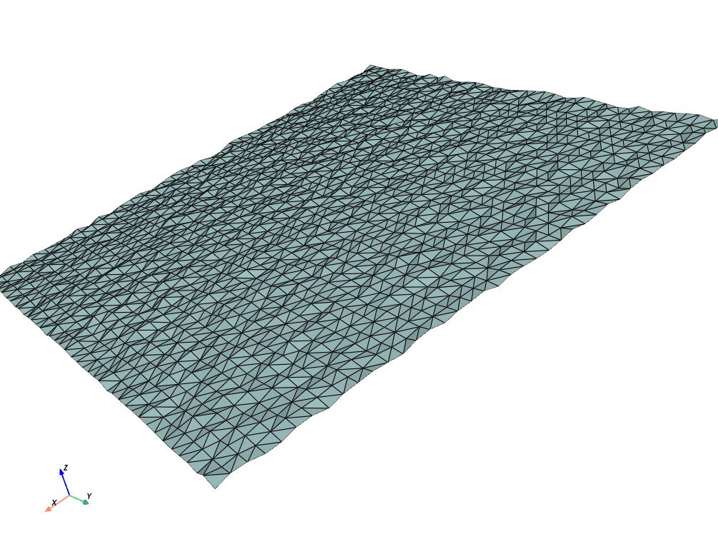
The purpose of setting up a 3-d connectionist neural network in the traditional way, is to create the coordinate space within which we embed our computational meshes. This way we can calculate vertex locations and the orientations of faces and normals. Such coordinate spaces exist in multiple domains, at multiple levels of resolution.
The connectionist network provides essential infrastructure for the computations that need to occur at the level of the mesh. In real biophysics, as it applies to both theory and real-world practical applications like medicine, these levels of description are inseparable, and real understanding (and modeling) involves the ability to move seamlessly between the levels. For example if one is trying to understand the effect of a drug on the brain, one must have some knowledge of where and how the drug binds (which neurons in what brain areas, and where the receptors are in those neurons), and how those binding locations affect the behavior of neurons in the network, and how that relates to the behavior of the organism. The point of the above simple presentation, is that the 2D grid representing a "sheet" of neurons is fundamentally no different from what we do with meshes. Just as we can divide a computer screen into pixels, the medical imaging community divides MRI scans into volume elements called "voxels", and surface elements are nothing but the boundaries of voxels, and voxels can be reconstructed from surface elements if we know which side is the inside. If you're way ahead of this discussion and terms like discontinuous Galerkin and flux reconstruction ring a bell with you, you're in the right place, hang out for a while and we'll have some fun. Meanwhile there's a lot of very bright biologists who haven't been exposed to this material, and as soon as they get their hands on it we'll see an explosion of new research. So let's finish with meshes, then we'll talk about how to make them watertight and computationally useful for studying things like astrocytes.
The square "sheet" of neurons shown above was conveniently aligned along the Z axis. We could, however, add a random offset to each Z coordinate, so the result looks more like a terrain (or perhaps a patch of membrane). Then, we can triangulate the resulting set of points to generate a computational surface. For example, if the cells are arranged in a 2-d grid the Z coordinate can be converted to an activity level, and thus the surface can show us the terrain of activity in the network. But this is a different representation from a grid, because now we have the concept of the "difference" between neighboring points. Depending on the model in play, the difference can become computationally significant, like if we have gap junctions between neurons. If this were a patch of membrane, we would have an inside and an outside, the surface would be oriented and we can use the spatial information to calculate physical properties of each little triangle. These calculations end up being pretty simple, because of the simplicial structure of the mesh. There is rarely a need to perform any actual calculus, most of what we do is simple addition and multiplication.
Here is a tracing of the proximal portion of an astrocyte. This came from an SWC file, which is a set of vectorized line segments with diameters. How do we convert this into a useful computational mesh? We can't just apply a Delaunay method to get triangles, because the computer doesn't know what part of the mesh is the inside. So we have to do a little pre-processing to get this mesh in shape. We have to calculate the normals attached to each piece of the surface, and orient the faces of the mesh correctly. Basically, we have to tell the computer a tree's a tree, otherwise it'll try to treat the branches like one big gigantic surface, and the calculation of the nearest neighbors along the boundary will go awry.
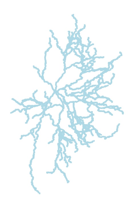
To see what this format actually is, we can zoom way in and look at the way the information is being represented for us.
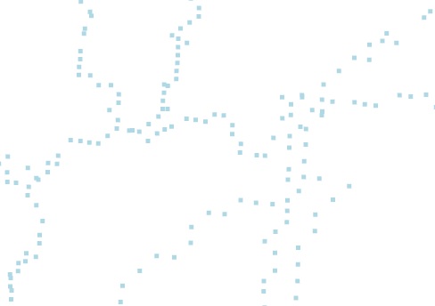
Aha! This is just a bunch of points, whereas the skeleton is built with vectors from one point to the next. This kind of silliness is absolutely typical of the state of the ecosystem in neuroscience, and it's one of the things Annie is here to address. (Go ahead and try to find an SWC file converter on Google, Allen has about half of one and BlueBrain has one but it's buggy and neither retains object identities, the SWC file defines a single object and there's no way to put any endoplasmic reticulum inside your neurons). To get a proper mesh from this file, we have to read it in a special way, because there's no way to get the geometry we need from a point cloud. When we read the SWC file, each vector has to become a cylinder, with the designated radius, starting from the parent location and ending at the tracing point. Keep in mind that we'd like to model a tiny section of this astrocyte, much smaller than anything represented in this file. So the mesh we seek has to subdivide each cylinder into computational compartments, and we'll end up with more compartments than we started with. To convert this file to a proper watertight mesh we have to trace around each cylinder, then combine the cylinders. Yikes! Look what happens when we do that, the cylinders need to be joined at every branch point. Here's just five of them near the soma.
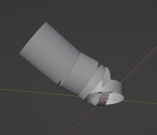
So we have to do a little work, shaving off the places where the cylinders overlap and joining the disconnected edges (and adding faces as needed). There are other ways of doing it, we can voxelize the image and resample it, basically put a new skin on it. But Annie has a magic method, that works every time, regardless of the size or quality of the input file. This is the result when Annie gets done with her magic:
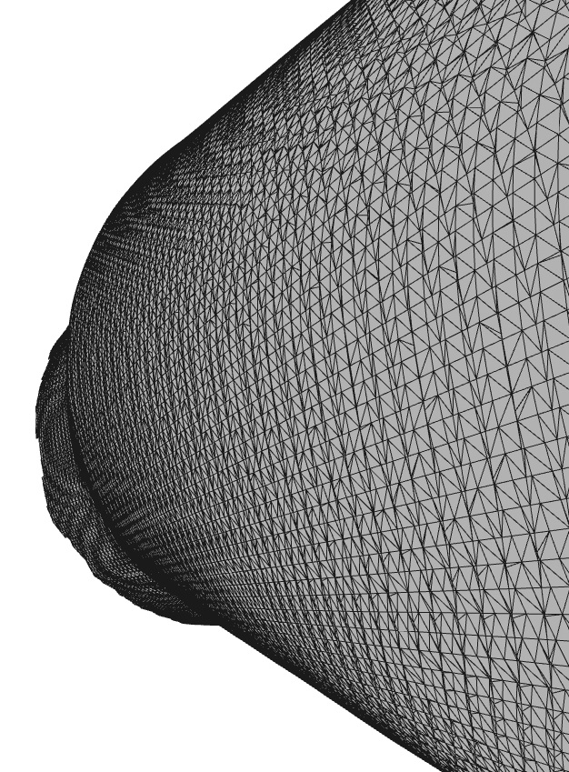
The resolution of this mesh is much better than 1 nm. What you see here is a tiny little piece of the traced astrocyte containing a branch and an end joint, no more than 0.1 micron in length. The entire mesh is completely watertight, and has been subdivided into perfect computational compartments. There are zero dangling edges and zero disconnected vertices, and zero faces that can't be computed. Every one of the 171,000 triangles is properly oriented and computationally accessible. When saved at maximum resolution there are over 100 million computational compartments in the finished mesh. Each one is just slightly bigger than the size of a glutamate molecule. From here, we can decimate down to any desired level of resolution, in favor of computational resources or to check discretization errors.
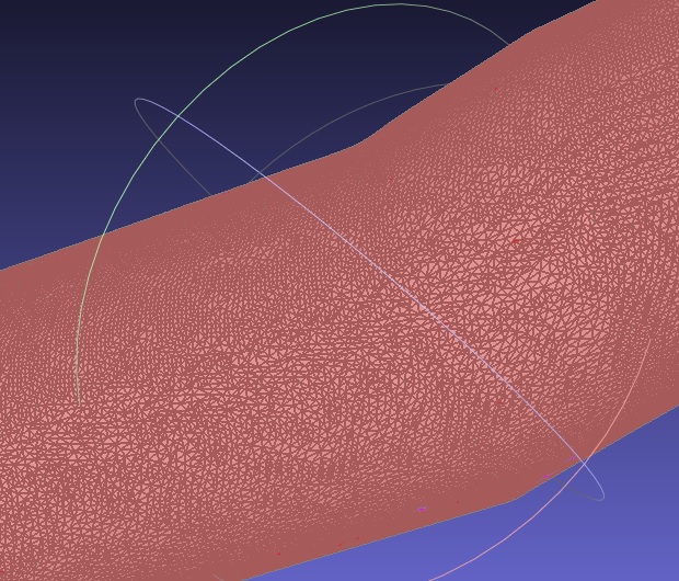 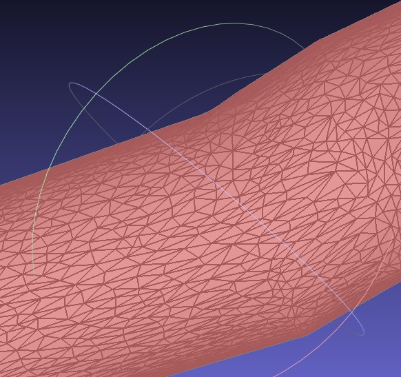 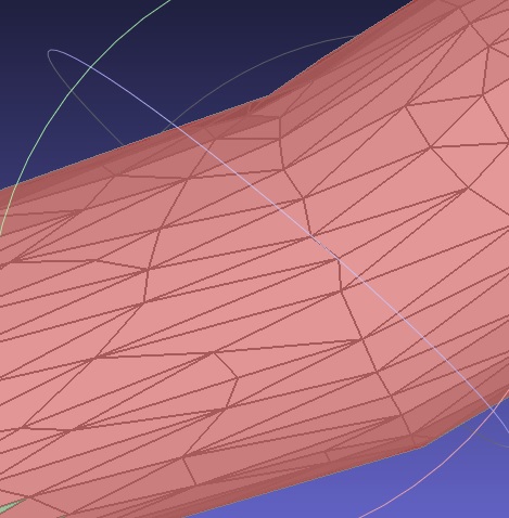
Visualizing a neuron from an SWC file is pretty easy, but turning it into a computationally useful mesh is another story. A computational mesh is a bit different from NEURON's idea of "compartments", and Annie lets you move seamlessly between the two interpretations. For biophysical purposes, a computational mesh requires the ability to attach physical materials to mesh elements. This in turn requires the mesh to be treated in a special way. Even a perfect triangular mesh is not enough, we need to compartmentalize the mesh and define how the boundaries behave. This concept is a little bit different than populating a membrane with a bunch of ion channels. For example, inside a neuron or astrocyte there are patches of cytosol with different physical properties, some have cytoskeleton which makes them more rigid and viscous, others have internal membranes that may involve elasticity and may or may not be attached to regions of the larger cytoskeleton. Annie can create computational geometry from pictures, from Neurolucida images, from SWC skeletons, from Blender, from EM stacks, manually, and synthetically. The starting material doesn't have to be perfect, Annie will heal the mesh and build a working computational structure, and populate it as needed for whatever biophysical purposes are at hand. On the next page we'll look at tracing and creating a neuron manually using Blender, and subsequently we'll see how to convert any such input into a working biophysical mesh using Annie's tool kit.
|