Meshing Requirements


A brain has a tight geometry, at any level of resolution. It forces us to discard the convenient physical assumptions of homogeneity and isotropy. When we say "multi-physics", we're talking about tiny polarized water molecules only a few Angstroms big, and glutamate molecules that are about 0.8 nm long navigating through an intercellular cistern 10-20 nm wide, with a bunch of big negatively charged cell surface proteins in the way. Water flowing through the cerebral vasculature creates a small percolation that causes charge layers to form in sheets, and the water flow ends up being laminar too. These features become computationally significant when we're talking about the attachment of transport proteins along the cytoskeleton, or the clustering of IP3 receptors on the internal membranes of the endoplasmic reticulum. We'll begin to see how that happens on the next page - and how shape at the microscopic level affects geometry at the macroscopic level, and vice versa.
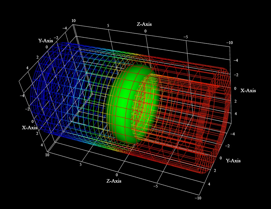
This is a computational mesh. It is somewhat more sophisticated than the simple cylindrical axons we created from definition files or from pictures. This axon is divided into computational compartments. You can see that the outer membrane now has 5 layers, and there is some kind of disc-shaped object inside the cylinder (maybe a piece of endoplasmic reticulum?), that's in a position to regulate longitudinal flow. The 5-layer outer cylinder can be used to position a lipid bilayer and some ion channels. We can increase or decrease the resolution of this mesh at will. The salient features are the surfaces and the small volume elements. In simulations, the volumes become dV and their boundaries become dΩ. On a discrete mesh we can define a patch of boundary simply by circulating around the nearest neighbors of a vertex.


Whether we're talking about heart valves, or cerebral vasculature, or the flow of water and hydrated ions through microscopic spaces, the principles are the same. In practice we're computing discrete differential geometries, and we're only limited by the computing resources available to us. However the models have to be correct! They have to accurately reflect realistic conditions. What is "realistic", how is that defined? Sometimes it's easier to define what's "not" realistic. At one level, the picture above looks like a cylinder, and one could sprinkle ion channels along the surface to acheive an "average channel density" that mimics biological measurements. However at another level that's unrealistic, because ion channels are spatially organized along the membrane, they're attached to the cytoskeleton and synaptic scaffolding. In many cases this organization is very specific, for instance the channel composition of apical tufts of cortical pyramidal cells is very different from that of the dendritic shafts. You may have noticed the saccules of endoplasmic reticulum in the picture on the Home Page. This kind of meshing is difficult to achieve, and it's even harder to place the IP3 receptors into the ER and anchor them in place.

Let's look at how we get from "neurons as spheres", to "neurons as meshes". Typically in biophysical experiments we begin by being interested in a small patch of membrane. Computationally, we need high resolution in this area, and maybe we don't need such tremendously high resolution in peripheral segments. If we're looking at a dendritic spine we may not care very much what the axon does, it just has to provide a stable sink for currents and a stable concentration of ions. We can therefore decimate the mesh in peripheral areas, and perhaps refine it near the areas we're interested in. On the other hand, if we're looking at ephaptic coupling we may care very much what the axon does, and in that case we may want the mesh to extend at high resolution all the way to the tip of the axon. This presents some scaling issues, and multiplying compartments is computationally expensive. One usually scales to the limits allowed by one's computational resources.


Branching Trees


The "branching tree" associated with axons and dendrites usually has sophisticated geometry, and it requires us to perform all manner of solid body transforms to extend the processes at the proper angles. There are many ways to ask Annie to build a tree for us. The general algorithm is that the axon travels forward a certain distance, then branches, and the branching is characteristic. From the standpoint of fractal geometry this is a straightforward procedural algorithm and all we have to do is specify the diameters of the branches. We can do this manually, we can provide Annie with some arrays: one that tells her when to branch, another than tells her how, and a third that tells her how much variance to apply to the branchpoints - and perhaps a fourth that attaches some variance to each branching operation. The result can be very realistic, although by using a predefined algorithm we're losing control over the dynamics. This is the manual way:

CELL XYZ
...
      NEURON_SIZE (5,5,5)
...
      AXON (5,5,0) CYLINDER * this tell Annie where on the neuron to position the axon
      BRANCH [ [(0,0,4000)], [(200,10,0),(200,-10,0)], [(100,10,0),(100,-10,0),(100,-10,10)] ]
      DIAMETERS [ 100.0, 80.0, 60.0 ]

We can do approximately the same thing in a single line of text using a FRACTAL directive or by pointing Annie to an external branching function. One of the neat things Annie can do is move axons around. For instance in the earlier example on the previous page, some "random paths" were shown that ended up traveling directly through neurons and such. We can prevent this by collecting the axons into a BUNDLE and specifying the bundle geometry. We can also use an AVOID_COLLISIONS directive when building the connections, which works better in close situations when bundles don't apply. In the context of an optic radiation, we'll probably want to define a bundle, that way we can do slick things with the visualizations, like color-code the topography. These capabilities are only a short step away from dynamic models of axon and dendrite growth, as we'll see below.

The problem with visualizing long axons is they're tiny! The neuron may only be a few microns wide, and if we attach an axon that's a micron wide and ask it to travel 10 cm, it will be hard to visualize, because it'll look like a tiny little thread in a sea of ... whatever else is there. Sometimes the diameter of an axon can be even smaller than that of a dendritic spine, there are many excellent reconstructions of axons climbing up the shaft of a dendrite and contacting its spines along the way. Here's an example, it's very hard to see the axon in a large coordinate space but when we zoom in everything's fine.


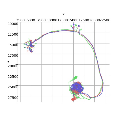
Here's another example, this is a Navis mesh, generated by tracing neurons. The axons are generally long, and we may wish to save some computation time by modeling the axons in a different way from the cell body or dendrites. On the other hand, axons are often "assumed" to be homogeneous, and that is not always the case.


It is important to understand these are computational meshes, the smooth surfaces are discretized and every vertex has data attached to it. If we're using a mesh to model the stresses on a beam, we can use a structured grid to position the vertices, and in that case mesh generation becomes a trivial exercise. However in neuroscience we have to build computational compartments from arbitary geometries, and calculate the currents between each compartment. And it gets worse - compartments are kind of a primitive way of representing axons and dendrites, more likely they're closer to one of Ilya Prigogine's experiments in nonlinear thermodynamics, where every point is an oscillator and one needs to model the coupling on a lattice before one sees the covariances that contribute to the spatial patterns. (A similar situation applies to Kuramoto oscillators created by neighboring ion channels, which has become a hot topic lately, especially as the behavior may relate to dynamic neural fields - and note the similarity of the figure in the middle of the link, to the self-organizing spatial patterns in the Belousov-Zhabotinsky reaction). Realistic simulations of axons show beyond any shadow of a doubt that the shape of the action potential is considerably different at the synapse than it is at the axon hillock. Branch points may lead to reshaping or complete failure. In practice, the mesh tool ends up becoming your best friend, because the ease with which you can manipulate geometry directly determines the duration of your workflow. To prove this to yourself, try calculating the number of ions that have to flow through a small patch of membrane to support an action potential, in two spherical neurons of size 1 micron and 10 microns. Now do it for a pyramidal neuron and a generalized (asymmetric) polygonal neuron of the same volume.

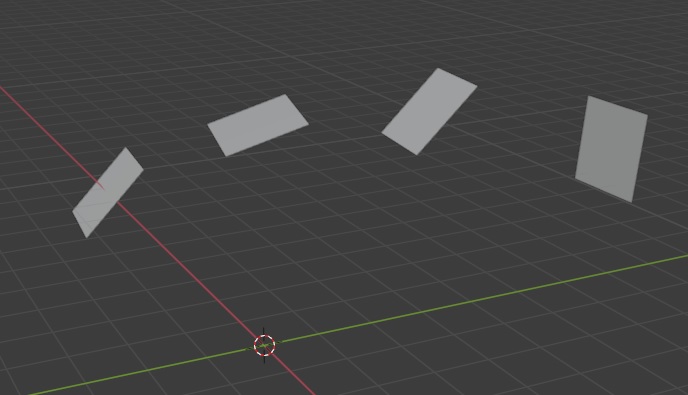
A quick word then, about connectivity. The basic connectivity of neurons is conceptually straightforward. Many people in the simulation world are used to working with 2-dimensional "sheets" of neurons, so here are some sheets of neurons:


They all have different orientations in 3d-space, just like they do in a real brain. And, if we want to connect them together topographically, we need to be able to map one plane to another. That's pretty easy, right? We've already seen how to define the geometry of a "sheet" of neurons. Like this:

CELL NAME c CENTER (800,200,300) EXTENT (500,500,0) ORIENTATION (20,40,60) ARRANGEMENT GRID_2D N_NEURONS 100

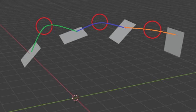
Some complexity arises with the connections. We'd like the axons to travel along well defined pathways, and they have to maintain their topography while they do that. Thanks to the connectome community we're fortunate enough to be able to directly map many synaptic pathways, however in simulations we're often interested in the physical movement of components (this is especially true in developmental scenarios). Here's an example:


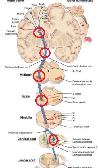
The nerve fibers have to travel through the areas defined by the red loops. To Annie, a collection of red loops is a BUNDLE, and each loop is defined the same way a CELL is, with a center, an orientation, and an extent. In the above picture there are three bundles of nerve fibers. Annie has further modifiers (like if you want an ellipse instead of a circle), or you can drag any object into Blender, modify it, and re-import it. So for example, here is how we might define a corticospinal tract, we basically just draw a few circles in the right places:


When the geometry gets tight, no problem. Axons can turn on a dime, just put your constraints at right angles and Annie will take care of the rest. This provides a simple and intuitive way of guiding axons along a path. Sometimes it provides a useful alternative to the idea of defining axons with a branching tree. You can use osculating circles too, to define the curvature in a slightly different way. There are also interesting branching situations like the optic chiasm, where half the fibers go in one direction and half in the other. This piece of development has been well studied and involves interacting protein gradients that align the source and target coordinates. Accordingly, more advanced instructions to Annie might include attaching chemical gradients to each constraint in a BUNDLE, and BUNDLEs are frequently found to terminate in NEUROPILs, which is yet another piece of chemically sensitive connection geometry. For this example bundle, to illustrate the concept, all we need is:

BUNDLE CORTICOSPINAL_TRACT
      CONSTRAINT CENTER (1000,1000,400) RADIUS 200 ORIENTATION (30, 20, 5)
      CONSTRAINT CENTER (6000,800,1400) RADIUS 400 ORIENTATION (60, 120, 0)
... etc

At the connectionist level we can call these "constraints", but Annie treats them like geometric markers with functions attached to them - and the functions operate on the mesh. You can see how this concept naturally dovetails with the chemoaffinity models related to development. With a CONSTRAINT, axons have to travel "through" the loop, whereas there are variations of another directive called EMIT, that push the axons "away" from the loop. One does this exactly like real brains do it, one places markers at various points to guide the axons along a path. Annie's EMIT directive uses an attached function to emit the marker, and another neuron (or astrocyte) can SEEK to it, and then various things can happen depending on the function. In the mesh, all the calculations and attached functions get converted into a very large system of differential equations, which is solved either internally or with a user defined solver. (Annie can use any solver known to Python, and then some).

There's a further issue with topographic mapping. Let's say you begin with a 2-d "sheet" of neurons, a typical "layer" as they say in TensorFlow, although that usage differs from the anatomical meaning. Typically you'd align the layer along one of the axes, like in the retina model shown earlier, where all the "sheets" of neurons were aligned along the Z axis. But now let's say you want to give one of the sheets an orientation, say, rotate it by 30 degrees on the Y axis (30 degrees of "roll"). The question is, do you want to map the topography before the rotation, or after it? Both conditions exist in the brain. In the case of the retina, we want to do it before, because even though the retina is a curved structure, the topography is essentially two dimensional. As we move centrally, more interesting things happen, for example in the optic radiation the actual mapping becomes somewhat logarithmic, Schwartz described it as a complex-log (like a seashell) but it's essentially an expansion of the foveal region. Annie will do whatever you ask her to do. She works much like Blender does, she can apply transformations after the fact, so for instance if you tell her GRID_2D and LAYOUT (10,0,10), that's where's she'll put your cells, but that's in "internal cell coordinates". When you specify an ORIENTATION you're doing it relative to network coordinates, so there's a transformation that takes place. One reason Annie keeps your original coordinates around is for the developmental scenarios, when things have to move. Having access to the original coordinates as well as the current coordinates is sometimes helpful. Another more basic reason is for handling mesh computations, because sometimes that needs to be done on the basis of geometry and sometimes there are additional aspects to it. In any case, you can map connections "into" a structure or "through" it.


Meshes and Connections


Ultimately, when modeling neural networks, we're interested in biophysics and biochemistry - the concentrations of ions on either side of a membrane, and the opening and closing of ion channels. In the last few years much of this landscape has been studied and charted. There are dozens of kinds of ion channels, some are voltage gated, some are rectifying in one direction or another, and some are linked to receptors that modulate their behavior. In some cases there is competition between ions for space in a channel, and there is a non-zero probability that neither ion will make it and the channel will open without consequence. When visualizing, we rarely look at the opening and closing of individual channels - instead we're usually interested in a local membrane potential or the spatial distribution of calcium ions. These are "derived" properties, they need to be computed. The general method for doing this, is to attach data structures and equations to each point in the mesh - then the simulator traverses the mesh and performs the calculations. The simulator doesn't know or care about geometry, it just crunches numbers. We have to set up all the geometry ahead of time, and provide the simulator with the proper descriptions so it can apply the math. A full description of discrete differential geometry is beyond the scope of these pages, for those who are interested in the underlying math I can highly recommend two collections of YouTube videos, one by user eigenchris covering tensor calculus, and another by Prof Keenan Crane at Carnegie Mellon (link below). An understanding of (discrete) differential geometry is important when working with finite elements and related models.

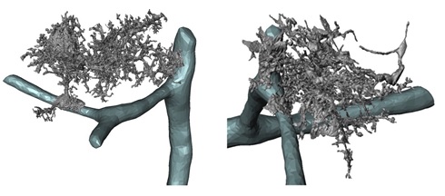
The cells in a mesh obey physical laws. The calculations we perform use Newton's and Maxwell's equations, and sometimes we have to deal with curvature which can be as tricky as relativity. The good news is, the physicists have already been all over this territory and they know what works and what doesn't. The big deal in neuroscience, is the boundaries. Boundaries exist at the edges of topographic networks, and they also exist along every single membrane in a nerve cell, including the interior membranes like endoplasmic reticulum. (ER has a membrane potential too, which is still difficult to measure and visualize with current technology). For computational purposes, one of the interesting questions is how to treat a boundary. Do you make it "infinitely thin" like a shell, or do you give it some volume? If you give it volume, you have to calculate what happens inside the volume, which means additional computation time. How you handle this depends on your simulation. Generally speaking, anything you care about should be calculated, it shouldn't be abstracted away. For example, Annie wants to look at astrocytes, which wrap themselves around synapses, thereby creating a very tight and very small extracellular space. Computationally this means non-homogeneity, which means we need a fine mesh to get any accuracy. But there's more to it, because if our extracellular space were infinite and homogeneous we could model the neighboring neuron as spheres, but because of the astrocyte we can't do that anymore - the extracellular space is now tight and narrow, and its exact ion concentrations (including their spatial distributions) are being regulated by the astrocyte. So the presence of the astrocytes dramatically impacts the way we have to handle the neurons. These are astrocytes - in this visualization they're in gray, and the big blue thing is the dendrite of a neuron.


Quite a few scientists have already understood intuitively, that meshes are the preferred computational solution for biological simulation, and people have tried using discrete differential geometry with varying degrees of success. This paper out of Europe is an excellent case study. Listen to this:

"Because human datasets are far from complete, computational models can be used to fill the gaps caused by missing knowledge and propose specific functional hypotheses. Detailed neuron models can be reconstructed from digital morphologies to generate morpho-electrical equivalents, which can subsequently be endowed with cell-specific ionic conductances. Simulations of responses to current injection can then be optimized against electrophysiological recording templates to extract missing information about model-free parameters, such as maximum ionic conductances. In this study, we utilized high-resolution morphological reconstruction of human PCs and unique electrophysiological recordings obtained in acute cerebellar slices from post-surgical cerebellar specimens to generate detailed biophysical models. This allowed us to simulate the electrophysiological response of human PCs under conditions that would otherwise be impractical for the experimental assessment and evaluation of their dendritic complexity and computational capacity".


Sounds great, doesn't it? Right up our alley. Until you start reading about how they did it. In addition to all the complexity up until the point of microscopy (like patch clamp recordings and so on), they traced all the dendritic trees by hand using a Wacom tablet, then they had to use NEURON and BlueBrain to work bottom-up with the ion channels, and they didn't have any human data so they used data from guinea pigs. Then they wanted to look at dendritic spines, so they had to use special software that didn't work quite right and they ended up having to arbitarily correct the Z axis by a factor of about 15%. Next we have this inevitable line buried in the depths of the paper: custom-made Python3/NEURON 8.0 script. The simulator wouldn't do what they wanted so they had to write a custom script. Then at the end of the paper there's a whole list of additional tools that includes MATLAB, native Python, NeuroM, TREES, Vaa3D... you see the problem here. They're in the business of collecting software, like people used to collect vinyl records and DVD's. Fractal analysis of dendrograms has its own tool. Somehow they had to get the data out of one tool and into another, which must have been a special treat. And at the end of the day, what have they learned? The title of the paper is "Human Purkinje cells outperform mouse Purkinje cells in dendritic complexity and computational capacity". Gee, I'm amazed. All that work for this? :)

I'm teasing - and merely pointing out that the ecosystem of tools commonly used by neuroscientists is still stuck in the 90's. Kristof Koch was looking at neural noise on meshes in the 90's. Other people had that idea too, but back then it was supercomputers or nothing. Today, meshes are on the desktop, and there's no excuse for not using them. ParaView is a very popular desktop application for visualizing meshes. Maya can generate animated characters on meshes, complete with rigged skeletons with forward and inverse kinematics. You can make your neurons twitch. Meshes are actually very efficient computationally, the discrete differential geometry is covered very nicely in a series of videos by Prof Keenan Crane from Carnegie-Mellon. One just has to be aware of the mesh storage format, there are perhaps half a dozen in common use and about two dozen more for special purposes. Annie will figure out the format from the file extension or by reading the first few bytes of the file, but for instance there are several varieties of binary STL files and Annie isn't going to try to keep up with proprietary formats. If you're a scientist and you're invested in proprietary formats, you should cut your losses and make the move immediately. OBJ files are perfectly adequate for 3 dimensional solid modeling, whereas dynamic visualizations require the ability to add data to vertices. Annie lets you attach arbitrary data to mesh elements. You can use the data for any purpose whatsoever, like rendering in the GPU. The size of the data structure is limited only by the computer's memory, and if it gets too big you can move to the database back end which scales into the billions of elements.


Choice Of Mesh Size


Mesh geometry is so important, we're still talking about it. The triangulation algorithms come up with all kinds of oddball tessellations - can't we just start with a cylinder and partition it somehow? Sure, well, we already talked about the problem you'll run into, which is what to do at the boundaries. How to smoothen your mesh, to make it computable - and this in turn has a lot to do with your choice of mesh size. We can learn from computational fluid dynamics, where there is something called the Knudsen number, that tells you whether a continuum assumption is valid. If the mean free path of a particle is about the same as the scale of the mesh, then the discrete molecular nature of matter becomes important and continuum math won't work. To use the continuum, you have to choose a representative volume element that's neither too big nor too small. It has to be big enough to average over, and small enough for the average to make sense. A similar situation applies in neuroscience, when we have ion channels in a membrane. The density and effect of channels varies widely, and they coexist with all manner of other membrane bound molecules. Channels can be motile or not, sometimes they're bound to a perisynaptic matrix and sometimes they diffuse in the plane of the membrane. So if we're trying to model at this level, our mesh size should be chosen so that we have "enough" channels in a patch of membrane - and if the resulting level of resolution isn't good enough, then we have to go to a different model (like the fluid dynamic example, we'll probably have to switch to a statistical simulation). You'll know it when you find a mesh size that works, because there will be a well defined range outside of which the model will blow up (meaning the differential equations won't converge anymore).

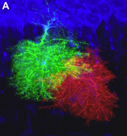
Let's use the astrocytes pictured above in a thought experiment. You see the one on the left, that looks like it touches the neuron in only two places, whereas the one on the right wraps itself around long segments of multiple branches. The dendrite itself is less than a micron in diameter, and the tiny feet of the astrocyte are no more than a tenth of that, maybe as small as 50 nm, or even less. Compare that then, with the size of a potassium channel, which is typically around 1-2 nm. In this case, a mesh size of 50 nm is too big, and 1 nm is too small. Let's try... 25 nm. That'll give us a few channels and it'll divide each foot into several compartments. The same approach can be used with synapses. So when we're building the mesh, we're not going to have any problems at the boundaries, because the mesh size is small and the junctions can be easily reshaped. On the other hand, we don't want to model the entire neuron this way, especially the long axon. So we ask Annie to decimate the mesh in the areas with the most uniform geometry (reduce the resolution by decreasing the number of computational compartments - it turns out that this is also an important trick in machine learning, where they call it something different). Here is an amazing fluorescent image of some calcium micro-domains in a pair of astrocytes. This is what we're trying to model. Take a good long look at this. The neurons are the big blue things on top, they're huge compared to the fine astrocytic processes, which are much smaller than synapses. The astrocytes wrap themselves around synapses, and a single astrocyte can have a million leaflets. Each leaflet regulates the extracellular environment around a synapse. Note that the calcium compartmentation unquestionably has shape. Some of the leaflets at the periphery are considerably brighter than others, indicating they contain more calcium. Are they sequestering it, or are they storing it in favor of synaptic activity? A good mesh model should be able to provide at least part of the answer. Microscopy might provide another part - are these micro-domains always associated with endoplasmic reticulum? If so, why are some leaflets brighter than others?


Neurons (and astrocytes) are living entities. They're not just numbers in a computational matrix. They move, they twitch, they talk to each other electrically and chemically. All of this is based on the same physical laws that form galaxies and spin planets in their orbits. When we observe a neuron, we do our best to "model" it, that is to say, try to describe it in terms of the laws we know about. This is how we arrive at a Hodgkin-Huxley equation, and it fits, it works. At a certain level. It completely fails at other levels, and students don't learn about that till much later. However neuroscientists know all about it, as transmission and communication is described in terms of probabilities, and the stochastic behavior of the elements. Sometimes, rapid fluctuations are abstracted away as "noise", and that's not always a good idea. Bandpass filtering a spike train means you'll never see anything outside of the band. We could spend several pages talking about noise (but we won't), because stochastic variation plays directly into the behavior of populations of neurons. Sometimes noise is necessary, the network won't work without it. Quantifying these relationships can be challenging. Even separating process noise from measurement noise can be challenging in a live experiment. If you're using a simulator to compare observed and theoretical spike trains, you'll probably be interested in the ways in which the simulator can mimic the "noise" you're seeing in the live signal. Noise relates to stability as well, and we're interested in stability because of things like epilepsy. The simulator is here to help us put together working physical descriptions, so we can create better technology and better analytical methods. The math is what enables all this, and the good news is it's actually very easy. You don't have to solve complicated surface integrals, the computer will do that for you. In the context of a computational mesh, we're interested in what goes in and what comes out of each compartment. The laws of physics are pretty simple in this case, if what came out is less than what went in, the rest must still be inside.

So let's talk some math. Here's a hot tip. If you've studied linear algebra and calculus and need a refresher on geometry, start here: How Long Is The Coastline Of Britain? This is a paper by Benoit Mandelbrot, the godfather of fractal geometry. To grasp differential geometry, one has to wrap one's mind around the concept of the "dual", and the answer to the question is, it depends how long the yardstick is. (The "measuring device"). If your yardstick is long, you'll measure as the crow flies and miss a lot of the details. If your yardstick is very short, you'll measure along all the jaggies and your answer will be bigger than if you'd used the long yardstick. The measuring device is the "dual" of the thing being measured, and in differential geometry we take advantage of this relationship by treating differential k-forms like yardsticks. If this is new to you, find the videos by eigenchris and Keenan Crane, and watch them a few times. Complicated-sounding differential operators like the Laplacian turn into sparse matrices this way, and the mathematics on the mesh becomes straightforward.

Let's play a game. What do you see here?
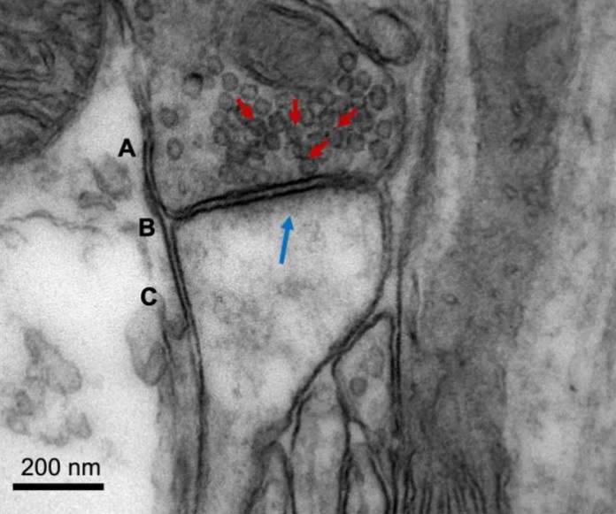

(Figure from Serrano et al 2022)

If you said "a synapse", or "a dendritic spine", you're right on target. You see the presynaptic vesicles, and you see the characteristic shape of the spine. But... what else do you see? Look again:
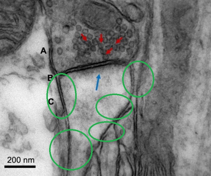


The synapse is surrounded by astrocytes. The junctions seem to be associated with endoplasmic reticulum in the interior of the spine. They're also associated with an intercellular web, as you can see especially clearly in the green circle on the top right. Dendritic spines are known to be extremely sensitive to local calcium concentrations, and astrocytes regulate local calcium through a complex biochemistry that ultimately involves processes in the interior of the cell (like IP3 receptors in endoplasmic reticulum). There is no doubt whatsoever that astrocytes affect synaptic function, this has been investigated in a myriad of ways and the results are consistent. So how come none of the simulators deal with astrocytes? The big hint is, the leaflets are too small, they can't resolve things that small. But Annie can! Annie will resolve computationally down to about 10 nm, which is about 1/10 the width of a small synaptic web. And that turns out to be just the about right size for realistic and provable models of astrocytes and neurons.

The point of all this, is that meshes have many requirements that go well beyond a simple surface representation. Depending on how ambitious we'd like to be with our biophysics, we may even wish to model the growth of axons as they find their targets, a process that involves filopodia on growth cones, the staging of internal and external chemical markers, and the effect of calcium on the cytoskeleton. To ensure that our geometry is working, we can test some forces on it. A simple experiment might be, isolate the tip of a dendrite and stimulate it electrically and chemically. This is easy to accomplish with a traditional simulator, but the results aren't very realistic. We're after realistic results. We don't want to have to tell the simulator what the equilibrium potential of a neuron is, we want the simulator to arrive at it on its own. To get a biophysical simulation to the level of a traditional simulation is a lot of work. The best traditional simulators have libraries of ion channels that can be assigned to computational compartments, but these libraries don't often translate easily into the language of biophysics. One finds in practice that one must frequently build suitable bio-materials from the literature. This is especially true for the cytoskeleton and other mechanical components that aren't usually represented in traditional simulators. To proceed from here, we'll need to survey a little math, because we'd like to understand the differences between finite elements, finite volumes, discrete differential operators and basis functions. This knowledge will be essential for us to perform meaningful calculations on a mesh.


All Right, Let's Do Some Math

Back to the Home Page


(c) 2026 Brian Castle
All Rights Reserved
webmaster@briancastle.com