The meat of a computational mesh is the idea of breaking up a surface or a volume into small elements. It's the same principle as calculus, where "d"x is used to represent an infinitely small increment. However continuous calculus in three dimensions is hard, it takes the CPU a long time to compute analytic solutions. On the other hand, a mesh is a "discrete approximation", and in that way it's almost like a "d"x, in that it gives us tiny increments that provide smaller errors than big ones. Meshing is a science unto itself. It's fundamentally based in discrete differential geometry, and it should be stated up front that a solid understanding of linear algebra is essential for theoretical neuroscience. A basic foundation in differential geometry and tensor calculus is highly recommended. There are some excellent resources on YouTube (referenced below).

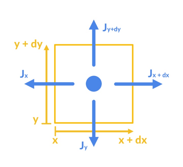
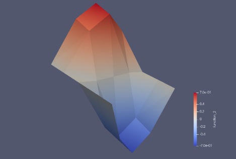
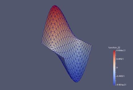
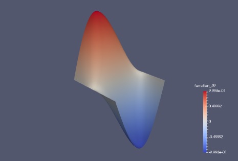
This figure below shows a piece of mesh with some geometry and some forces. In this case it's a square, and in three dimensions it might become a cube. We can use this cube to approximate a tiny piece of a neuron or astrocyte surface. We'll get some approximation errors, which we can minimize by making the cubes very small. This principle is shown with triangles on the previous page, and in general we can use any polyhedral form (some are computationally nicer than others, triangles and squares and their N-dimensional extensions are industry standard, there are only a very few cases where we require something more). For our purposes we'd like vertices that are affinely independent, which means we prefer triangles to squares and tetrahedra to hexes.

Already at this stage, we should be aware of the math we'll need to make our simulations work. For computational purposes, there are some tremendous advantages in using discrete differential geometry rather than traditional finite element methods. We'll discuss these in more detail when we get to physical materials. The tradeoff has to do with the way the mesh is represented in the computer's memory. Either way, the discrete geometry allows the computer to conveniently calculate small increments piece-wise rather than having to integrate and differentiate over continuous domains. In general we'll have some kind of function (or combination of functions) over the geometry, like we might have an electric field, or we might have some regional ion concentrations, and we might even be interested in the velocity of water as it flows through a mesh element. We can approximate the function(s) of interest using a set of basis functions, so the field becomes a linear combination of basis fields, and then all we have to find is the weights to assign at each point in space. If the basis functions are precise enough, we can interpolate the values between the vertices and arrive at a smooth approximation to the actual function, and in general if the mesh has enough resolution this approximation will be very good. Generally then, we have a shape, and some functions on that shape.



(Figure from SimScale Wiki)


Some of you (those who are reading carefully) may have asked, "wait... you were showing me spherical neurons but you told me spherical neurons are bad". So, okay... let's look at some neuron geometry. The essential need in the workflow is to create realistic geometry either synthetically or from microscope images. Annie can do both. On the previous page we quickly showed the synthetic concept, on this page we'll quickly show the microscope concept, and then we'll move on to begin discussing the computational geometry of the mesh, and why it's meaningful for things like astrocyte-neuron interactions. The first goal in the finite element workflow is to create a useful mesh, regardless of the starting point. It must be computationally watertight, and it must accurately represent our geometry.

There are three important concepts to understand up front: one is, neurons scale up, and scale down. Any time we're talking about a neuron, we're talking about little tiny ions that cross a little tiny membrane. And, we're also talking about millions upon millions of these neurons, organized into interconnected populations. A simulator needs to be able to zoom in and zoom out, and ultimately the limit of precision depends on the ability to represent a floating point number in the computer. The IEEE 128-bit format gives us 35 decimal digits, whereas ordinary floats of the Python type give us about 15 digits, and in real life the precision is about half of that (because two small numbers multiplied together should still yield a non-zero result).

The second important up-front concept is that generating a computationally useful mesh is an iterative process. Even if you start with a "theoretically perfect" mesh, it may or may not be computationally useful for you, depending on what you're trying to do with it. A big part of this has to do with boundary conditions, the mesh must be "shaped" so as to accommodate realistic boundary conditions, and it must also be "scaled" so the mesh size is neither too big nor too small. There is no "one-button solution" to this part of the workflow, although ANNIE comes close. Typically one must iteratively "curve fit" to different mesh sizes and boundary conditions, to attain working computational geometry, and Annie helps you do this quickly and interactively. Once the mesh is inside Annie, you can do a lot with it, but here we're still talking about the starting point. Different people do this different ways, we're showing a synthetic approach and a photographic approach which are probably the two most common ways in practice, and Annie accommodates these workflows and more, because she understands the goal. Theoretical perfection is not the goal - computational utility is the goal. (It would be a bit arrogant to assume theoretical perfection in any aspect of modern biophysics - typically models last about ten years, and those with extended longevity sometimes have names like "Nernst" and "Stokes" attached to them!)

The third important up-front concept is that meshing separates geometry from topology. This is actually one of the big reasons we use meshes, neuroscientists need to understand the significance of such a separation, as it becomes very important in areas like information geometry. In a mesh, surfaces and volumes are divided into tiny pieces with straight edges. There are vertices, edges, and faces, and they obey Euler's formula. Each vertex has a location, but the location is separable from the connectivity. We can define the connectivity of a vertex without ever referencing its location or the locations of its neighbors. Two essential concepts that arise are distance, and the physical variables that are being calculated, which end up being attached to mesh elements. Each vertex, each edge, and each face, has data attached to it. The specific data varies according to the simulation. Sometimes it will include a trans-membrane potential, other times (like during developmental studies) there may be a moving physical location (which means, a dynamic mesh with vertex locations that change with every iteration). What the simulator does, is calculate the value(s) attached to each mesh element, at every point in (simulated) time. The solver uses constraints based on physical laws, to convert a set of partial differential equations into a set of ordinary differential equations, which can then be quite easily solved on a mesh. (If you're a machine learning engineer, you may be familiar with the physics-informed neural networks that estimate the parameters in such arrangements. We'll have quite a bit to say about this when we get to information geometry).

What Is A Computational Mesh?

In a computational mesh, we divide the surface and/or volume into discrete partitions and imagine that there is some kind of function overlaid on them, like maybe an electric field or the local concentration of calcium ions. We could have a scalar field that only has one value at each point in space (like the calcium concentration), or we could have a vector field that has a sophisticated spatial behavior (like the flows of calcium ions from one point to another). We use the laws of physics to understand that the calcium that exits a volume, minus the calcium that enters it, must still be in the volume. Thus any volume can become either a source or a sink for the flow of calcium ions. And when a charged particle moves from one place to another, there is a current associated with it, and if all the movements are aligned (like, transversely across a cell membrane) the currents add instead of canceling out. So we have charges moving around, at the same time we have particles moving around in a viscous fluid, and these are constrained by passive processes at the boundaries including porous ion channels, as well as active processes including voltage gated channels, pumps, and exchangers. The purpose of the mesh is to allow us to calculate all this stuff. The more "stuff" we have to calculate, the more degrees of freedom we'll need, and the more demanding our computations will become. Even a coarse mesh can have hundreds of degrees of freedom, and we'll probably have to restrict our enthusiasm and relegate some of these to the "statistical approximation" corner, unless they're directly germane to what we want to look at. Such approximations use "lumped" parameters, and this technique works to varying degrees depending mostly on the system dynamics (it worked well enough to get Ilya Prigogine a Nobel Prize in the area of nonlinear thermodynamics).

To make the simulation work, we have to define boundary conditions, which are constraints on the equations. For example in physics there is the concept of a "wall", which is a boundary. With a perfect wall, gas molecules simply bounce off, but there is also the concept of an imperfect wall, for example in acoustics we have semi-reflective walls that absorb part of a pressure wave, and this behavior requires a description of the boundaries in terms of one set of constraints as distinct from another (Neuman vs Dirichlet, Robin vs mixed, and so on - if you're new to this, you'll understand what these terms mean before we get done). With neurons, a logical boundary is the semi-permeable cell membrane, and we also have the issue of objects within objects - for example there are all manner of organelles inside a cell that also have membranes, like mitochondria and endoplasmic reticulum, and we need to keep these objects separate in our calculations because they may have very different properties. The basic idea is pretty easy, we're going to take our cell and divide it into computational compartments, and any place there's an internal object it'll be defined by a boundary, and the entire neuron will have a boundary too. Specialized membrane structures (like gap junctions and the synaptic scaffolding) will be handled by altering the local properties of the compartments within our mesh, so in addition to the variable we're most interested in (like calcium concentration), we'll have a whole host of other variables we'll need to track, and this could potentially become a very large array, depending on how many degrees of freedom our computers can reasonably handle. We'd like to track "everything", but this is not feasible - at some point our computers will begin to complain, or simply shut down. So we'll calculate as much as we can, given our computational resources, focusing on the most important and most significant parameters.

What is true with meshes, is we can easily change their resolutions. The computation time is directly tied to the mesh size. The larger the compartments, the faster the simulation will be, and the more error it will have. With small compartments, the simulations will be a lot slower but considerably more accurate. Where along that spectrum you end up, depends on your scientific need. And usually, simulations that demand accuracy proceed through initial stages that don't, in other words it may take some time to find the parameter space that works the way you need it to, and you might start with a coarse linear simulation to show you the overall shape of the result, and then refine it in increasingly complex steps as it becomes more resolute, then nonlinear, and eventually stochastic.


           
(Figures from Imperial College London GitHub Site)


So let's start from the beginning. Before we can even tell Annie to go populate an array of neurons, we have to know what the neurons look like, and in most cases this starts with a microscope image. In biological tissue neurons are visualized by "staining", a concept that now includes fluorescent markers that can respond to calcium concentrations and membrane potentials in real time. The accuracy of the shape of a model neuron is determined by how precisely we can stain it, and then how precisely we can see the result in the microscope. Staining (also called "labeling") has gotten pretty good, there are specific proteins that can be attached to membrane objects to visualize them at very high resolutions. The microscopes are also very good, but the stains and the microscopes don't always work together perfectly. Sometimes we can stain things we can't see, and vice versa. So in addition to tracings and 3-d computer reconstructions from serial sections of microscope images, there are heuristics and assumptions that guide our choices, and they need to be exposed and addressed. Let's use an example, we'll create a computationally meshed neuron from a photograph.

When we're talking about spherical neurons, that's "a" starting place. Lego neurons are in fact an excellent starting place, for many kinds of geometries. Let's take a look at some other starting places. A common workflow in neuroscience is tracing a neuron in a microscope. Neurolucida is a popular and powerful software for this purpose. It exports data files that can be directly read into ANNIE. But let's back up a minute, because this is worth looking at in some detail. Coordinates in ANNIE are defined in terms of a "cat's-eye view", so the negative X axis is to the left, and the positive X axis is to the right. Similarly, the negative Y axis is down, and the positive Y axis is up. The positive Z axis is farther away from the cat, so "farther away" from the retina. The negative Z axis is behind the cat. This reference frame allows the convenient definition and calculation of linear and affine transforms, like roll, pitch, and yaw. But different software treats the coordinate axes differently, and it is important to be aware of the coordinate system used in the data source. ANNIE can re-orient as needed for an import or export, but you have to tell her which direction is up, otherwise she won't presume to alter your data.

To illustrate a tracing and mesh building workflow, we can use a popular (open source) mesh tool called Blender to implement a poor scientist's version of Neurolucida, and the reason it works is because at the end of the day, Blender exports the same files that Neurolucida does. Importing and exporting from Blender is exactly the same as importing from Neurolucida (the power and value-add of Neurolucida is on the front end, on the microscope side). To illustrate this we've built a model retina inside Annie, consisting of 14 cell layers, with a remote light source and a projection into the lateral geniculate nucleus (LGN). The definition file is here. It's a simple geometry, we aren't trying to model the optic chiasm. We simply have some sheets of neurons arranged within a coordinate space. When we export this network from Annie in Wavefront OBJ format, and then import it into Blender, Blender shows us exactly the same objects as Annie does.



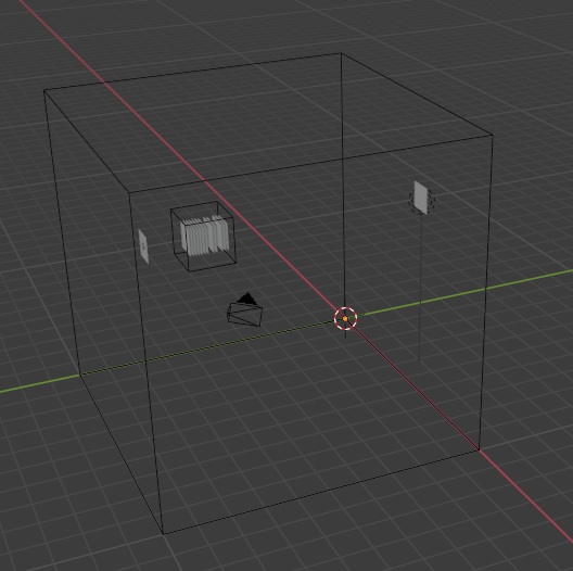
We can then make full use of the convenient toolsets inside Blender. Here is what our retina looks like, viewed from afar, complete with light source and a remote sheet of LGN neurons. Here we're displaying the network in wire frame mode, whereas the individual cell layers are shaded.



Networks and neurons can be created inside Blender (or any other mesh tool, including professional CAD tools like the Autodesk suite, and even gaming tools like UnrealEngine), and imported into Annie. You can get very specific with the geometry this way, you can define the shapes of cortical sulci and gyri if you wish, using splines or NURBs or meshes any other method the visualization tools will support. In the unlikely event that you can define them analytically by providing equations, Annie will handle that too. This is one of the beautiful things about meshes, you don't have to worry too much about equations describing your surfaces, you can simply draw them. If you have equations, you can use them, but the mesh doesn't require it. Let's take a look at the Neurolucida workflow using Blender. We're going to trace the neuron starting from a picture.

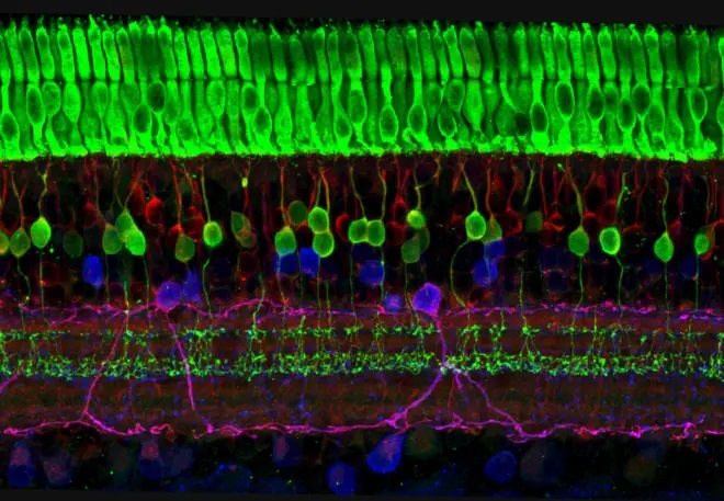
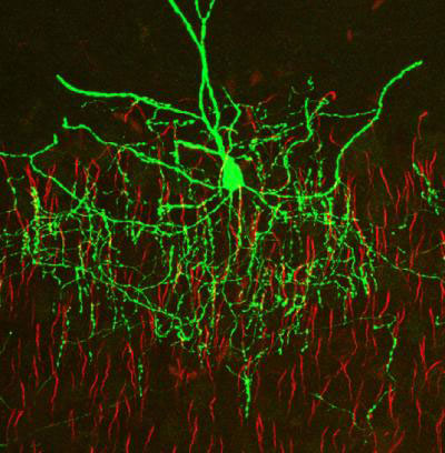
Some of you may have been laughing at the Lego neurons shown earlier, because real neurons are considerably more complicated. For instance here are some real neurons, the retina is on the left (you can see the beautifully layered neuropil), and a cortical chandelier cell is on the right.


Let's create a meshed neuron inside Blender, from one of these photographs, and import it into Annie. Here's an elementary trace of a neuron, showing the outline of the cell body, and we've asked Blender to put a thin cylinder wherever we trace an axon or dendrite.




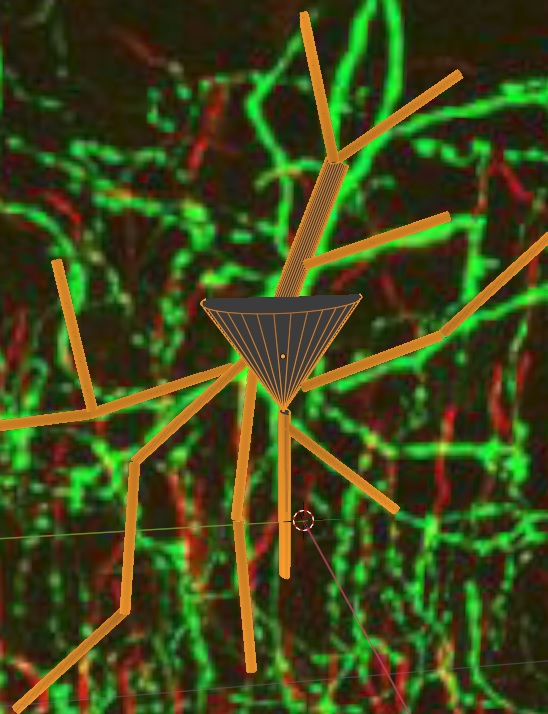
After achieving a suitable neuron, we can ask Annie to replicate it for us, with or without variance, and populate the geometry of our choice with the instances. From the standpoint of simulation, this level of description sometimes results in computational complexity with questionable benefit. Lego-type neurons are often quite sufficient, they can be generated in seconds rather than minutes. However sometimes it is quite necessary to be specific, especially when we're trying to understand electrical behaviors related to geometry. Here is the same neuron, exported as an STL file and displayed in Microsoft's 3-D Viewer.


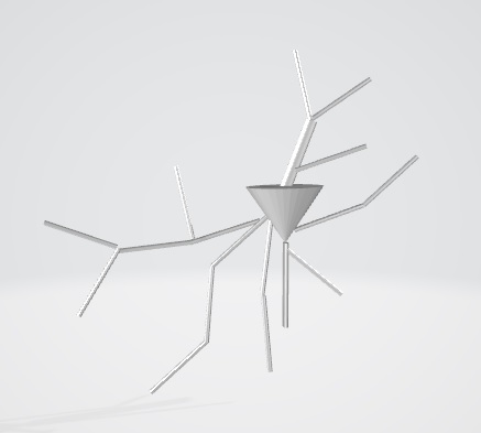
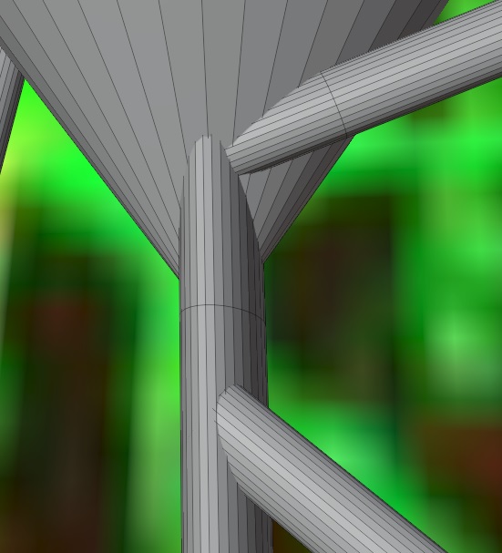
Apparently, Blender didn't do a perfect job of healing the mesh, but it doesn't matter. On the way back in, when this is imported into Annie, the faces will be reconstructed and the missing edges recovered. Here's the before and after. After Blender's "join" operation, the segments are joined but not necessarily in the right way.


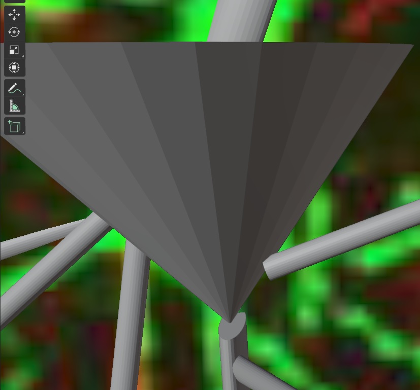
After importing the mesh into Annie, this is the result - Annie has extruded the required components and now she'll reposition the vertices just like Blender does, only she'll do a better job. Then she'll adjust all the places where the individual meshes meet, to make them smooth and computable. Then the mesh precision can be adjusted according to your computational needs. As with everything Annie does, you can be as simple or as precise as you wish, with your geometric definitions. If you care about compartment layout, you can pick vertices and move them around. If you don't, you can just tell Annie "give me surface patches about a tenth of a micron on a side, more or less". Really. It's that easy. Meshes made simple. Of course, you'll see exactly what the boundaries are doing when you visualize the results. Boundaries are a big deal in neural networks. One will notice them at the level of connectivity, and also at the level of the neural membrane and the contents of a cell. Biophysical characterization does not always align with simple symmetry. Neurons are not liposomes, they don't often have regular geometry.

Here's another interesting example, here we've imported a picture of a hippocampus, and arranged a curved plane in approximately the shape of the CA3 region we're interested in modeling. It was easy, just create a cylinder, rotate it by 90 degrees, and move it to wherever the image says it should be - then delete the bottom half and the two caps. Less than 30 seconds from start to finish. Now we'd like Annie to populate "this" geometry with 100,000 pyramidal cells, and connect them topographically into the subiculum. At this point, Annie leaves the others in the dust. No one else can do this, in 3 dimensions or even 2, but Annie can do it in about a tenth of a second. All she needs is another similar sheet that describes the target. So in less than a minute, you've created some realistic connection geometry, which you can then embellish with basket cells and granule cells or whatever else you'd like to include. Maybe you'd like to tweak the apical dendrites a bit and put some voltage dependent calcium channels there. Easy - select a channel by clicking on a vertex, make the modifications, and tell Annie to apply them to "all" channels - as is, with a function, with a map, with a gradient or with a computed mesh, and with or without a variance.





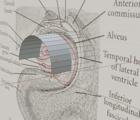
After making a few adjustments to the CELL definition, the result might look something like this:


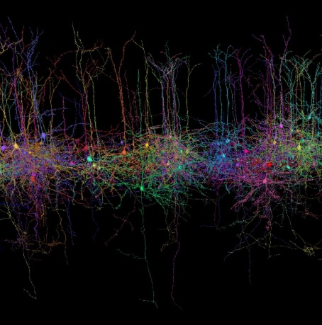
However this network is now more than just a photograph, each neuron is a computational mesh. Annie has an enormous library of dendrite behaviors based on channel placement, you can simply tell her that apicals are type 1 and basals are type 2, or you can get as detailed as you wish with specific channel positioning. Going straight from a photograph to a network is a slightly different concept than starting with a neuron tracing and then populating the shape of a cell group. At this point though, we've covered four different ways to create neurons, from tracings, from photographs, synthetically, and from text files. Regardless of the starting point, the network elements have to be converted into a form suitable for biophysical simulation. Some of that is merely vocabulary, but much of it is computationally meaningful, and some of it involves gathering information about materials from online (bio)-chemical databases.

The Blender neuron above, while representative in certain ways, is not biophysically realistic, nor is it computationally accessible. To get from a prototype to a computational mesh, we can take the source through several stages. First we can ensure that the mesh is watertight, by patching any holes and plugging any open endpoints. Then we'd like to triangulate the mesh at a fine level of resolution, but we can't do that directly because the branches only overlap by location instead of by vertex. There are several ways to get a better mesh, for instance one can sample the surface and then reconstruct it using a Poisson method or a metaball. We'd like the result to be regular, in other words it shouldn't have any exceedingly thin slivers or fantastically obtuse angles. These requirements are not necessarily easy to accomplish, the ecosystem of mesh tools is such that many tools will crash immediately unless they're given exactly what they want in exactly the right form. ANNIE's stragegy is to first create a standard intermediate form (like a Wavefront OBJ that's portable across practically every meshing application in existence), then build it up in stages until it meets the computational requirements for a finite element simulation. Along the way the intermediate stages are kept in various formats, including tetrahedra and voxels, and if the resulting meshes are good enough to be read into MOOSE or Elmer they're also good enough for one of ANNIE'S DEC simulations.

The idea of "healing" a mesh is very important. Neuroscientists don't have the luxury of dealing with regular structured meshes. Everything encountered in biology is highly unstructured. And, it's still pretty rare to be able to visualize an entire neuron in three dimensions under the microscope (lately the best successes have come from AI, using ANN's specifically trained to parse connections from electron micrographs). So when we're building a neuron from pictures, we usually begin with imperfect meshes, and when we put a bunch of imperfect meshes together, we end up with an even worse starting point. The concept of "aligning the meshes" is an important milestone for a network model, because we need computability. In the places where different kinds of meshes intersect, there has to be "regularization" applied to each mesh to generate computationally acceptable intersections. Many times we'd like to extrude a mesh to add additional structure to it, for instance if we'd like to represent boundary layers along a membrane, or frame a cytoskeleton underneath. If you're familiar with meshing, you may have heard discussions about the boundary layers, things like prism layers, inflation layers, and Y+ values. Annie is hip to all that, and if you're already at that level, these are some of the tools Annie can bring to the table for you:

• Classic Delaunay and Voronoi Tesselation
• Advancing Front Methods
• Greedy Meshing
• SVR (Sparse Voronoi Refinement)
• Marching Cubes, Surface Nets, and Flying Edges
• Poisson Surface Reconstruction
• Metaballs and Ball Pivoting
• Fast Quadrics for Decimation
• Extrusions and Refinements of all kinds
• Adaptive Meshing (in several flavors)

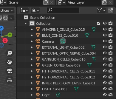
To introduce the concept of connectivity, here is an example of how even simple visualizations can help us right out of the starting gate. If we simply tell Annie to create some cell layers for us, without any further instructions she'll create them as rectangular grids (they show up as "cubes" inside Blender, as seen above). After a network build, all the synapses are in place and the underlying computational infrastructure is completely defined. When you switch to the "Neurons" tab, you might see a view like this:




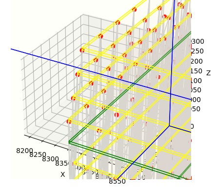
Here, we've only asked Annie to build synapses, without telling her how, other than by giving her the most elementary of CONNECTION specifications. Without further branching directives or a connection map, Annie will simply connect one neuron to another, and you can see the resulting axons in gray. The visualization helps us immediately, because one can tell at a glance the geometry is all wrong, there are fibers that travel right through neurons and all kinds of other non-biological horrors. However for computational purposes, this level of geometric non-sense might be okay, because we may not really care about the paths of the axons. However if we do care, we can ask Annie to fix these problems for us, by giving her slighly more refined CONNECTION directives. On subsequent pages we'll consider some of Annie's dynamics, because Annie will handle developmental scenarios too. Neurons that migrate, and connections that travel along specific paths. As always, these scenarios are described at a high level with simple directives, like BRANCH, SPROUT, EMIT, and SEEK. If you'd like your axons to climb up a gradient to find their targets, that's a one-liner in a definition file. If you'd like them to turn at a 120 degree angle at a specific landmark, that's another one-liner. These scenarios are taking us down to the biochemical level, so we'll look at some ion channels too, and we'll start talking about actual computations and what they look like on a mesh. Goldman and Katz look a little different there. The plasma membrane is a physical boundary between the intra- and extra-cellular environments, but it has complex geometry, there are Debye layers on either side of the membrane that can sometimes best be approximated by additional boundaries with distinct physical properties.

Historically, an early effort to link network morphology with network behavior is this paper out of the Blue Brain Project in Europe. The paper is titled "Reconstruction and Simulation of Neocortical Microcircuitry". It's an amazing piece of work, it really is. They were able to reconstruct an entire section of mouse brain in three dimensions, and relate it to the firing of neurons, in the 2015 time frame before AI burst upon the scene. After reading through this though, the question is: "where are the astrocytes?" They have lovely pictures of neurons, but no glia. And look how they had to view their results:



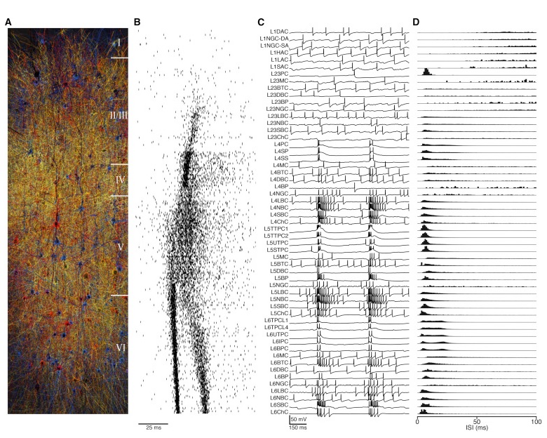
Today, just ten years later, we can do a lot better. With current technology we can easily generate animations like this, you can look at little patches of membrane in something approximating real time, see the fields and the ion concentrations at the same time:



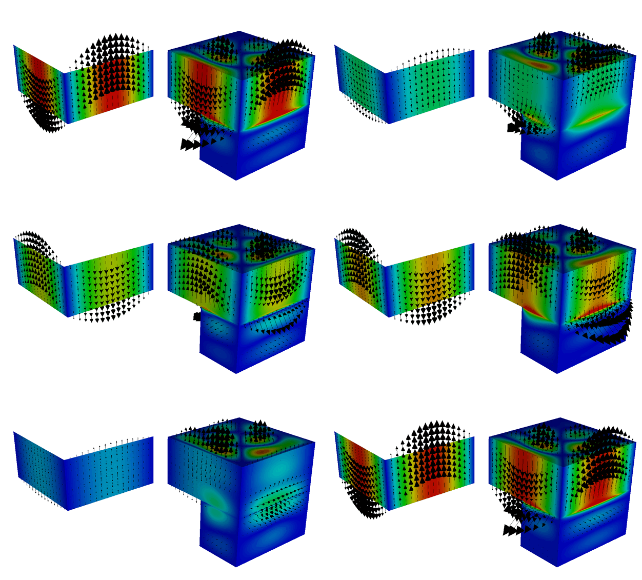
So how do we get from A to B? A better question is, how do we do it in a user-friendly way so Joe and Jane Scientist can work at home on their PC's without having to spend a lifetime learning other peoples' software and beating their heads against the wall when it doesn't work? In today's world Python presents a powerful scientific ecosystem, but getting data into and out of the various tools can be a considerable chore. There is an enormous library of neuron morphologies at George Mason University, but they've all been skeletonized in SWC format which most of the mesh tools don't read. And meshparty won't let you read in OBJ files from Blender unless they're completely perfect to begin with (you can't do what we just did above, drag in an imperfect mesh and fix it). So then you have to write some software to convert file formats, instead of spending your time on neuroscience. ANNIE was written by neuroscientists, for neuroscientists. ANNIE understands the workflows, and the objectives. When the above paper from Blue Brain was written, an existing neural network simulator was expanded to run on a supercomputer. In today's world there is the cloud, and you can have as many GPU's as you want just by asking for them. You can split up your workload over dozens of machines at once, for the most part computational power is no longer an issue. What is, is visualization. There's still a gap in the space between spike times and AI-generated images. How we get from A to B, is to fill that space. ANNIE believes this will happen automatically once the tools are brought from the supercomputer to the PC, and become easy to use. Let's look at how we can scale simulations from the near-atomic level all the way up to the whole brain, without making biologically unrealistic assumptions like isotropy and homogeneity.

How Did We Animate This Mesh?